Momentum contrast for unsupervised visual representation learning

BibTex
@inproceedings{he2020moco,
title={Momentum contrast for unsupervised visual representation learning},
author={He, Kaiming and Fan, Haoqi and Wu, Yuxin and Xie, Saining and Girshick, Ross},
booktitle={Proceedings of the IEEE/CVF conference on computer vision and pattern recognition},
year={2020}}

url= https://openaccess.thecvf.com/content_CVPR_2020/papers/He_Momentum_Contrast_for_Unsupervised_Visual_Representation_Learning_CVPR_2020_paper.pdf
Summary

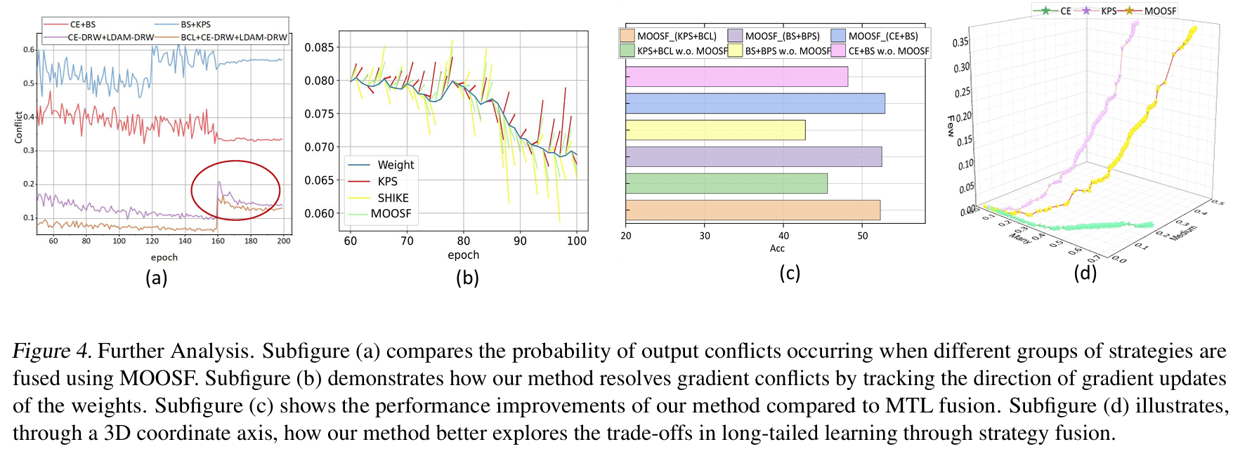
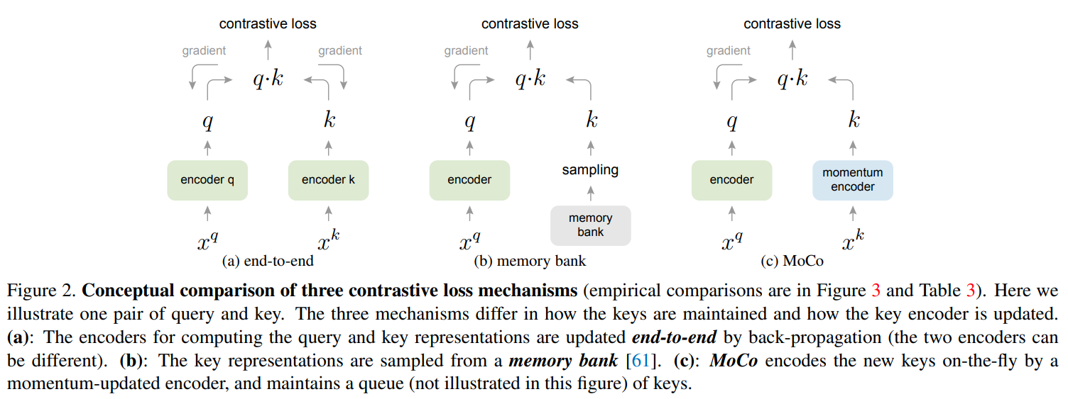
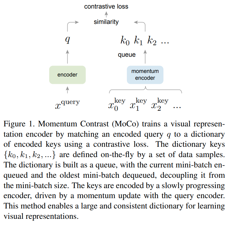
This paper is tackling the problem of representation learning with contrastive loss where an encoded query is matched to dictionary of encoded keys. Contrastive methods are sensitive to the number of negative examples, usually limited by the batch. Compared to previous methods such as end-to-end training of 2 encoders or using a memory bank, this paper proposes a new method called Momentum Contrast (MoCo) that uses a queue to store multiples batches of encoded keys in Fifo style and a momentum update for the key encoder to ensure all encoded keys in the queue belong to the same representation space. The queue overcome the limitated on the end to end technique which was limited by the overall hardware memory available for the batch and the momementum update ensure that the keys are in the same representation space unlike the keys in the memory bank. From training, only the query encoder is updated by backpropagation. The key encoder is conservatively updated by momementum update where at most 10% of the key encoder is updated by the query encoder. They notice Batch normalization is not effective in this case because it leaks information via intra-batch communication across samples. To fix that, they introduce Shuffling Batch Normalization where they use multiple GPUs, performing batch normalization on independly for each GPU and then shuffling the samples across GPUs.

Problem representation learning by expand negative pairs

Solution, Ideas and Why Fifo queue of multiple batches of previously encoded keys. the queue is larger than any single batch. Momentum update for the key encoder to ensure all encoded keys in the queue belong to the same representation space.

Images

A simple framework for contrastive learning of visual representations

BibTex
@inproceedings{chen2020simclr,
title={A simple framework for contrastive learning of visual representations},
author={Chen, Ting and Kornblith, Simon and Norouzi, Mohammad and Hinton, Geoffrey},
booktitle={International conference on machine learning},
year={2020}}

url= http://proceedings.mlr.press/v119/chen20j/chen20j.pdf
Summary

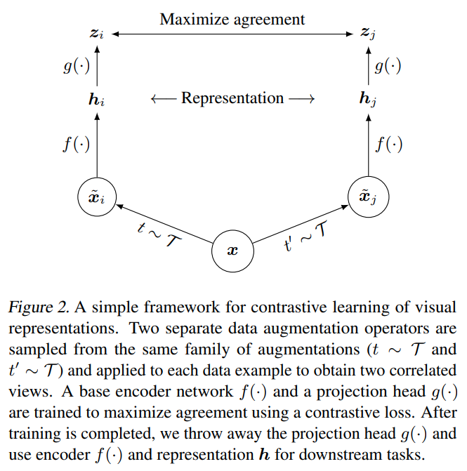
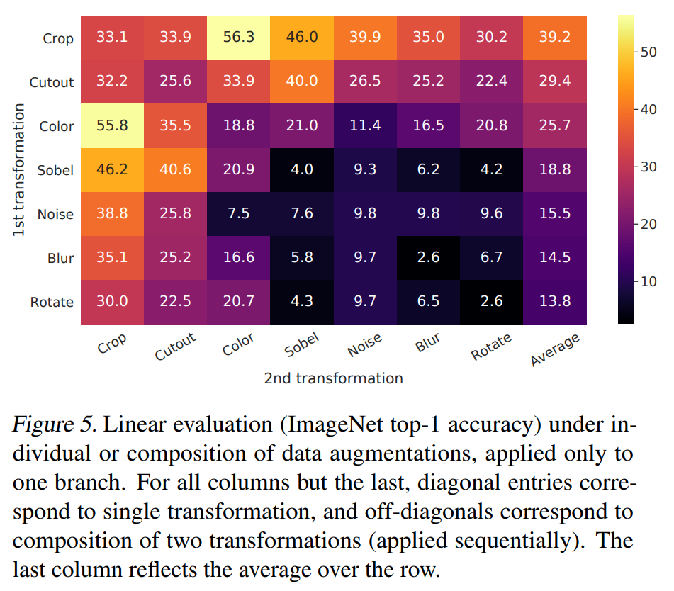
This paper tackles the problem of representation learning with contrastive loss. The paper proposes a simple framework called SimCLR that uses a non-linear projection head on top of the encoder to get an embedding that is contrasted with other embedding of the same sample. Given a sample, they apply a random composition of augmentations like crop, color etc to get a positive pair of augmented view from the same sample and contrast it with negative pairs of view from different samples in the batch. As such, the perform the best, the number of negative examples needs to be large, making the batch size large. They explored different combinations of augmentations and found that the best combination is a composition of random crop, color distortion, sobel filtering and gaussian blur. The introduced projection head as simple mlp before the contrastive loss to put distance between features and output so less information is lost in features. Overall, they found that introducing a simclr stage before finetuning the model on the downstream task improves the performance of the model.

Problem representation learning by expand negative pairs through data augmentation

Solution, Ideas and Why
Composition of augmentations like crop, color etc to get a positive pair of augmented view from the same sample. Contrast with negative pairs of view from different samples Add a projector (mlp) on top of the repr. encoder to get embeddings that will be contrasted. Puts distance between features and output so less information is lost in features. pretrain -> simclr -> finetuning

Images

Bootstrap your own latent-a new approach to self-supervised learning

BibTex
@article{grill2020byol,
title={Bootstrap your own latent-a new approach to self-supervised learning},
author={Grill, Jean-Bastien and Strub, Florian and Altch{\'e}, Florent and Tallec, Corentin and Richemond, Pierre and Buchatskaya, Elena and Doersch, Carl and Avila Pires, Bernardo and Guo, Zhaohan and Gheshlaghi Azar, Mohammad and others},
journal={Advances in neural information processing systems},
year={2020}}

url= https://proceedings.neurips.cc/paper_files/paper/2020/file/f3ada80d5c4ee70142b17b8192b2958e-Paper.pdf
Summary

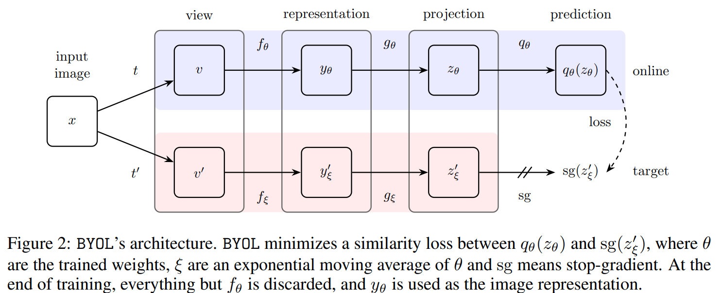
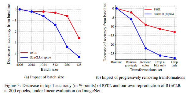
This paper tackles the problem of representation learning but with no negative pairs. The paper proposes a framework called Bootstrap Your Own Latent (BYOL) that uses 2 branches a momentum encoder, a projector head, a predictor head, and no negative pairs. BYOL works by 2 augmented views of the same sample, and passing to the 2 branches. The first branch has an online encoder updated by backpropagation that produces a representation of the augmented view. That representation is passed to the projector head which is a mlp that outputs a projection of the representation. Finally the projection is passed to the predictor head which is a mlp that outputs a prediction of the projection of the other branch. The other branch has a target encoder updated by momentum update that produces a representation of the other augmented view. The representation is passed to the projector head to get a projection of the representation. That second projection is the projection that the predictor head is trying to predict. The momentum update is a at most 10% update of the online encoder. BYOL uses symmetric loss, meaning that the augmented views are passed to both branches in the first order then the reverse order. This approach is at risk of collapsing to a constant function where all inputs are mapped to the same representation. To avoid that, they use the momentum update on the target encoder branch.

Problem representation learning with no negative pairs

Solution, Ideas and Why positive pair into 2 branches, one with encoder, projector, and a predictor learning to predict the projection of the other branch, encouraging same representation for positive pair. momentum update on the target network branch (no predictor) to avoid collapse of the network to a constant function give same representation for all inputs.

Images

Self-supervised relational reasoning for representation learning

BibTex
@article{patacchiola2020relational,
title={Self-supervised relational reasoning for representation learning},
author={Patacchiola, Massimiliano and Storkey, Amos J},
journal={Advances in Neural Information Processing Systems},
year={2020}}

url= https://proceedings.neurips.cc/paper_files/paper/2020/file/29539ed932d32f1c56324cded92c07c2-Paper.pdf
Summary

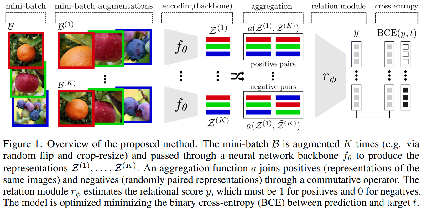
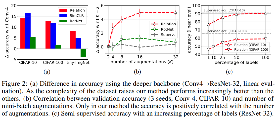
This paper tackles the problem of representation learning but with relational reasoning module and cross entropy loss instead of using contrastive loss. They propose a framework called Relational reasoning that uses a relational network to ingest concatenated positive pair from augmented view of the same sample and negative pair from augmented views of different samples. The relational network outputs relation probablity of a pair being related to the same sample. The relational network is trained with binary cross entropy loss. They explored different aggregation methods for the relational network and found that concatenation is the best.

Problem representation learning with 1 positive pair and 1 negative pair

Solution, Ideas and Why relational network ingest concatenated positive pair and negative pair. outputs relation probablity (1 for related, 0 otherwise). more efficient as the number of comparision scales linearly with the batch size (instead of quadratically), best aggregation is concatenation, loss is focal loss.

Images

Unsupervised learning of visual features by contrasting cluster assignments

BibTex
@article{caron2020swav,
title={Unsupervised learning of visual features by contrasting cluster assignments},
author={Caron, Mathilde and Misra, Ishan and Mairal, Julien and Goyal, Priya and Bojanowski, Piotr and Joulin, Armand},
journal={Advances in neural information processing systems},
year={2020}}

url= https://proceedings.neurips.cc/paper_files/paper/2020/file/70feb62b69f16e0238f741fab228fec2-Paper.pdf
Summary

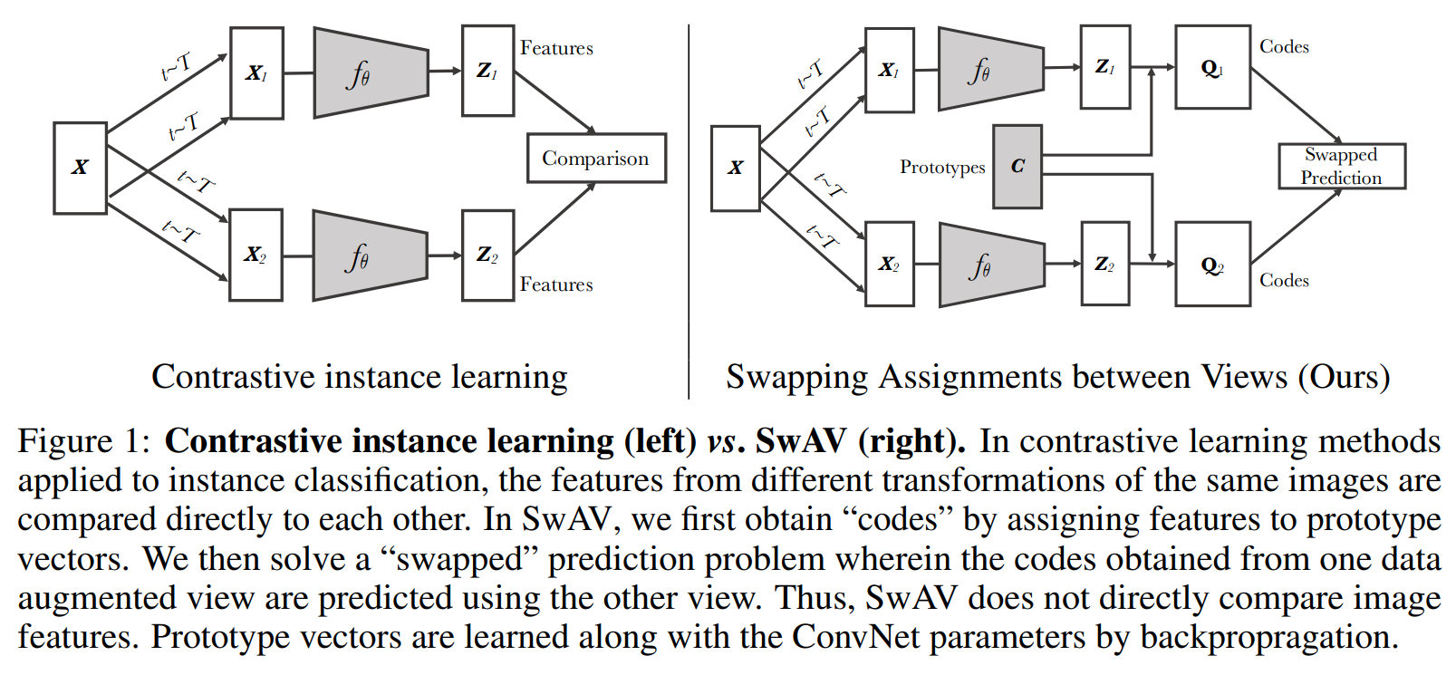
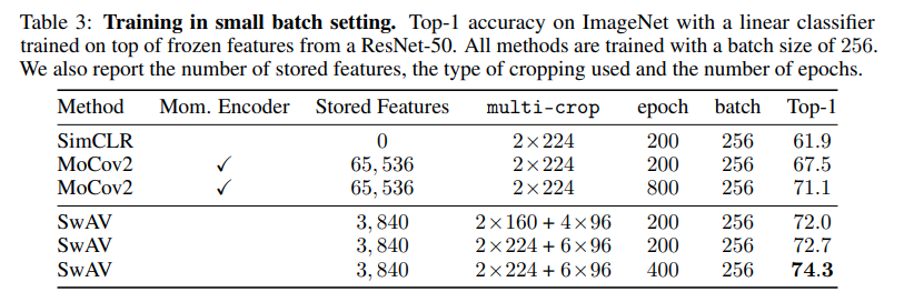
This paper tackles the problem of representation learning but with no negative pairs and no contrastive loss. The paper proposes a framework called SwAV that doesn't match projections but matches cluster assignments of augmented views. They start by learning cluster prototypes such that the cluster assignments of the positive pair of augmented views from the same sample are the same. Their framework consist of a 2 branch network. From a single sample, they produce 2 augmented views, pass them to the 2 branches. First the encoders of the 2 branches produce representations of the augmented views. The representations are passed into a projection head to produce projections of the representations. The projections are passed into a cluster assignment head to produce cluster assignments of the projections to the cluster prototypes. The loss function compares the cluster assignment of one branch to the projection of the other and vice -versa symmetrically. They also introduce multi-crop or using 2 standard resolution images and multiple low resolution crops to increase performance.

Problem representation learning with no negative pairs

Solution, Ideas and Why matching cluster assingments of positive pairs to learned cluster prototypes (symmetric loss). multi-crop or using 2 standard resolution images and multiple low resolution crops to increase performance.

Images

Vime: Extending the success of self-and semi-supervised learning to tabular domain

BibTex
@article{yoon2020vime,
title={Vime: Extending the success of self-and semi-supervised learning to tabular domain},
author={Yoon, Jinsung and Zhang, Yao and Jordon, James and van der Schaar, Mihaela},
journal={Advances in Neural Information Processing Systems},
year={2020}}

url= https://proceedings.neurips.cc/paper_files/paper/2020/file/7d97667a3e056acab9aaf653807b4a03-Paper.pdf
Summary

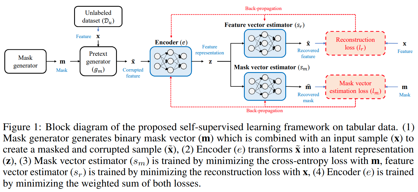
This paper is tackling the problem of representation learning with tabular data. The paper propose VIME or Value Imputation and masked estimation where there are a 2 stages, a self supervised stage and a semi-supervised stage. In the self supervised stage, they mask a random subset of features and then pass the corrupted sample to the encoder which then outputs a representation. The representation is then passed to a decoder which outputs a reconstruction of the original sample and another decoder which outputs the mask applied to the samples. The second stage is a semi-supervised stage where they create several corrupted views of the same sample and pass it to the encoder along with the original sample. The encoder outputs a representation for each view. The representations are passed to the predictor head to output predictions for the original samples and the corrupted views. The original sample prediction is compared to the original sample label and the corrupted views are compared with each other to make sure, coming from the same original sample, they are consistent in predictions. In total, the network has 3 branches and 4 loss functions. The reconstruction and masked estimation loss for the first stage. The Supervised and Consistency loss for second stage. The masking process is done by randomly shuffling the values of the features (columns) of the samples in the batch.

Problem representation learning on tabular data

Solution, Ideas and Why mask input samples and learn generative features to predict the original sample and the applied mask. in addition to supervised loss, use consistency loss that encourages same representation for augmeted views of same input

Images

Exploring simple siamese representation learning

BibTex
@inproceedings{chen2021simsiam,
title={Exploring simple siamese representation learning},
author={Chen, Xinlei and He, Kaiming},
booktitle={Proceedings of the IEEE/CVF conference on computer vision and pattern recognition},
year={2021}}

url= https://openaccess.thecvf.com/content/CVPR2021/papers/Chen_Exploring_Simple_Siamese_Representation_Learning_CVPR_2021_paper.pdf
Summary

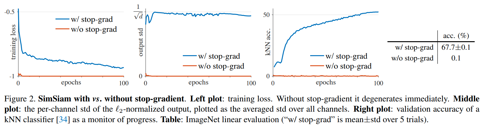
This paper tackles the problem of representation learning with siamese network and the collapse issue. The propose a simple siamese network that uses predictor branch and a non-predictor branch with stop gradient, no negative pairs, and no momentum encoders. From a single sample, they generate 2 augmented views and pass them to the 2 branches in both this order and the flip order of the views. Both branches have the same encoder, but only the predictive branch has gradient updates. the encoders output representation and on the predictive branch, the representation is passed to a predictor head to predict the representation of the second branch. The loss is a symmetric cosine simimlarity loss between the prediction of the first branch and the projection of the second branch. They show how their approach is similar to an expectation minimization algorithm and the stop-gradient is important to preventing collapse to a constant function.

Problem representation learning with siamese network simplified to avoid collapse without using negative pairs

Solution, Ideas and Why stop gradient in non-predictor branch to avoid collapse to constant function. symmetric (views are swapped) loss matching first branch prediction and second branch projection.

Images

Barlow twins: Self-supervised learning via redundancy reduction

BibTex
@inproceedings{zbontar2021barlow,
title={Barlow twins: Self-supervised learning via redundancy reduction},
author={Zbontar, Jure and Jing, Li and Misra, Ishan and LeCun, Yann and Deny, St{\'e}phane},
booktitle={International Conference on Machine Learning},
year={2021}}

url=http://proceedings.mlr.press/v139/zbontar21a/zbontar21a.pdf
Summary

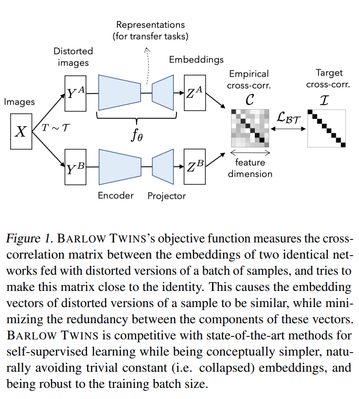
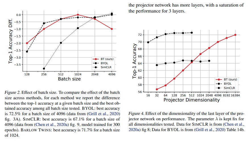
This paper tackles the issue of avoid collapse to a constant function in representation learning by measuring the cross correlation matrix. Given a batch of samples, they generate a random pair of batches of augmented views passed into a shared decoder and projectin head to produce a pair of projections of the batch of input samples. From the batches of projections, they calculate the cross correlation matrix between the 2 batches of projections. The cross correlation matrix should be an identity matrix meaning that the same feature indices should be correlated and different feature indices should be non correlated. To calculate the correlation, they assume the features are meaned at 0 over the batch dimension and divide by largest cross correlation value to avoid large feature values being interpreted as large correlation.

Problem representation learning without negative pairs and avoiding collapse

Solution, Ideas and Why cross correlation matrix loss between 2 views embeddings should be identity matrix where same features should be correlated and different features should be non correlated. the cross correlation calculations should include a normalization denominator so large feature values are not interpreted as large correlation

Images

Whitening for self-supervised representation learning

BibTex
@inproceedings{ermolov2021whitening,
title={Whitening for self-supervised representation learning},
author={Ermolov, Aleksandr and Siarohin, Aliaksandr and Sangineto, Enver and Sebe, Nicu},
booktitle={International Conference on Machine Learning},
year={2021}}

url=http://proceedings.mlr.press/v139/ermolov21a/ermolov21a.pdf
Summary

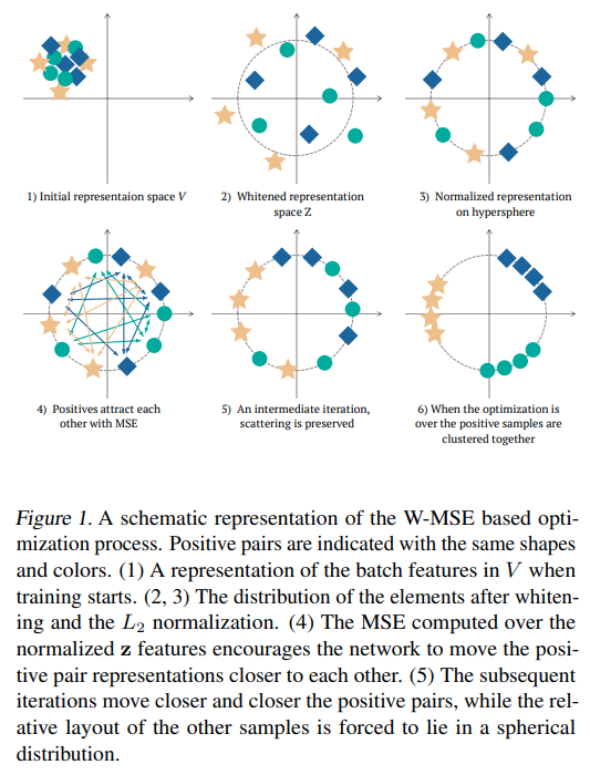
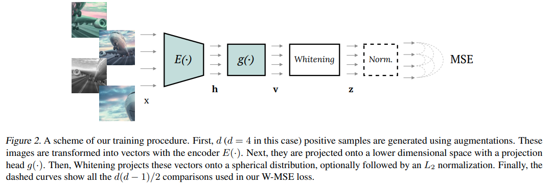
This paper tackles the problem of representation learning with whitening. The paper propose whitening to prevent collapse. The authors first start by producing a lot more than 1 positive pair with no need for negative pairs. They do that by augmenting the input sample multiple times and passing the augmented samples to the encoder to produce multiple embeddings. They then whiten the embeddings by moving them to a zero mean 1 standard dev distribution. Normalize them so they rest in a unit circle. Then they calcualte MSE similarity between all positive pairs to attract them together. The whitening step require calculating the Wv matrix and Mu mean of the embeddings. To better estimate Wv matrix, they partition the set of embeddings according to augmentation applied. Use same random permutation of elements across partitions to obtain subbatches. They calculate Wv and mu's for subbatches. Repeat this process to obtain decent estimates of Wv and mu's.

Problem representation learning with avoiding collapse, no negative pairs, and more positive pairs

Solution, Ideas and Why produce a lot more than 1 positive pair and whiten their embeddings by moving them to a zero mean 1 standard dev distribution. Normalize them so they rest in a unit circle. calcualte MSE similarity between all positive pairs to attract them together. To better estimate Wv matrix, partition the set of embeddings accroding to augmentation applied. Use same random permutation of elements across partitions to obtain subbatches. calculate Wv and mu's for subbatches. Repeat this process to obtain decent estimates

Images

Subtab: Subsetting features of tabular data for self-supervised representation learning

BibTex
@article{ucar2021subtab,
title={Subtab: Subsetting features of tabular data for self-supervised representation learning},
author={Ucar, Talip and Hajiramezanali, Ehsan and Edwards, Lindsay},
journal={Advances in Neural Information Processing Systems},
year={2021}}

url= https://proceedings.neurips.cc/paper/2021/file/9c8661befae6dbcd08304dbf4dcaf0db-Paper.pdf
Summary

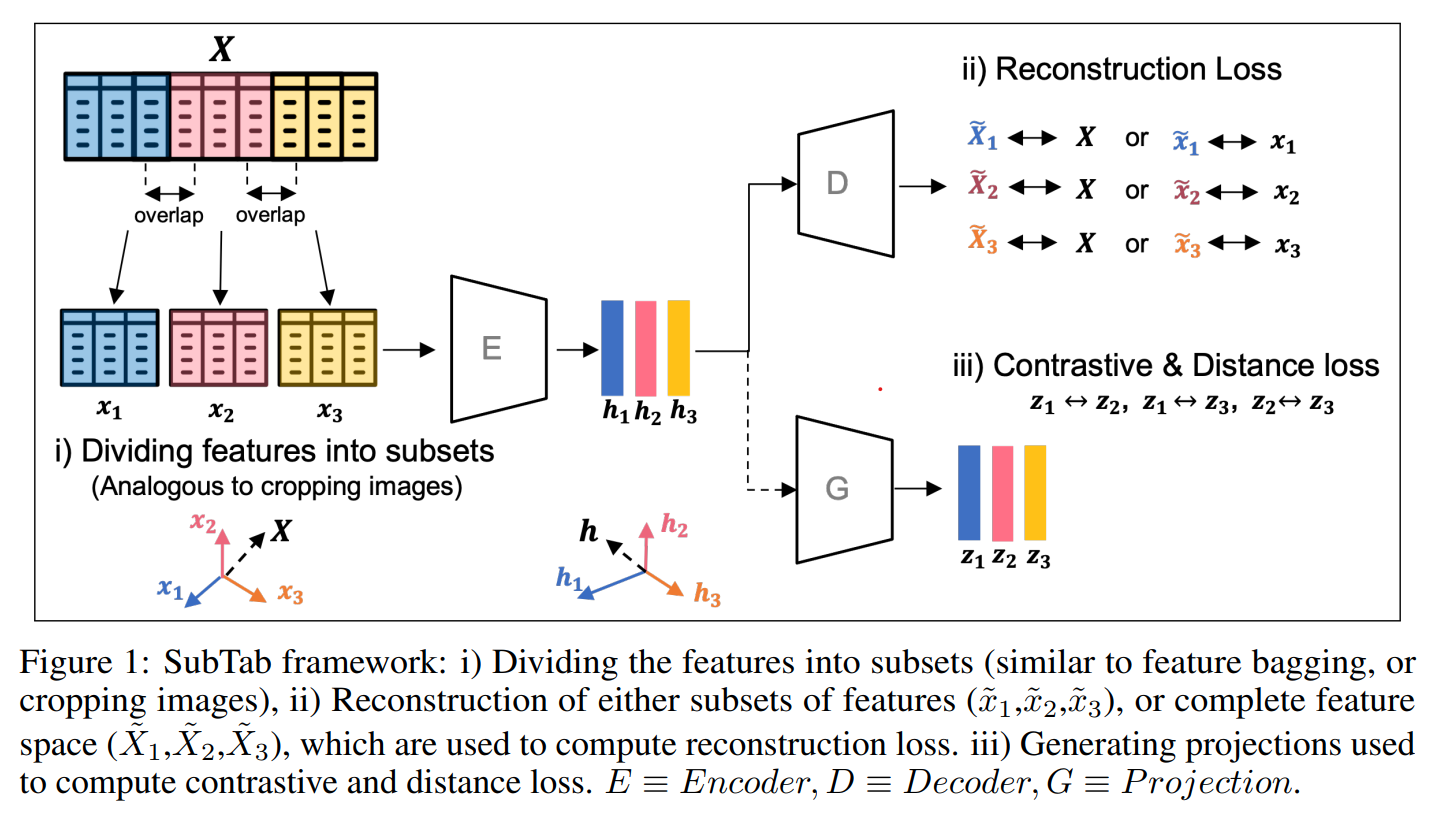
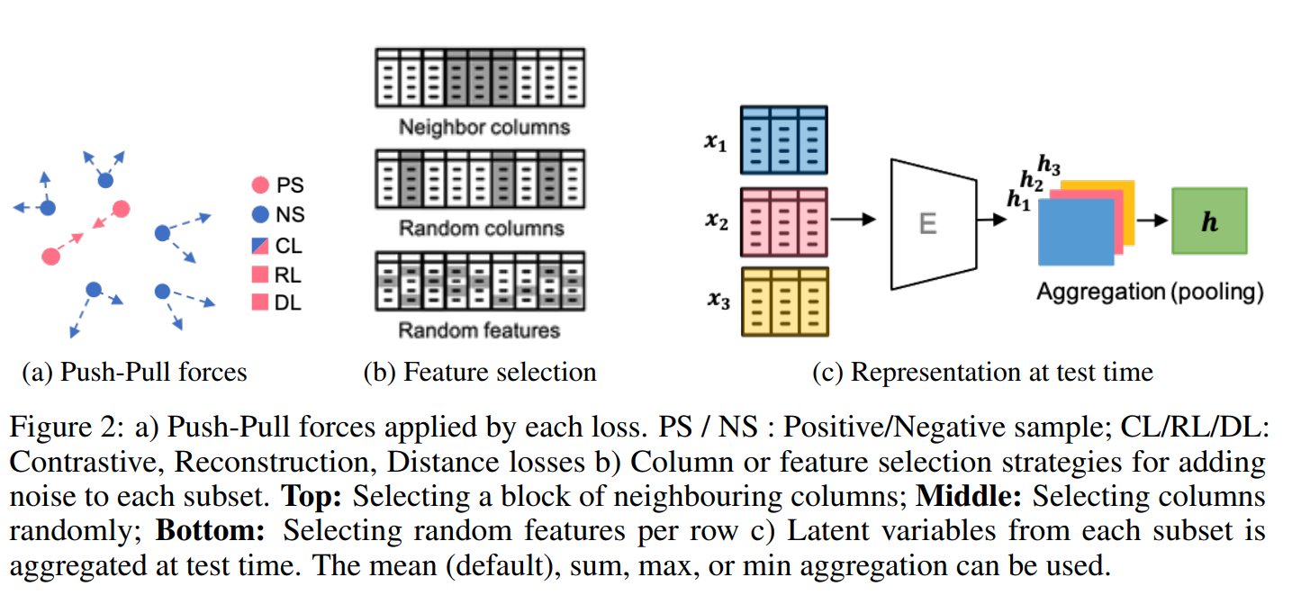
This paper tackles the problem of representation learning with tabular data. The paper propose SubTab or Subsetting features of tabular data for self-supervised representation learning. They divide the input instance into subsets. Subsets are used to learn representations that aggregated form the representation of the input instance. During training, the subsets are corrupted with noise. First the subsets were masked based on 3 masking schemes: 1. Random block of neighboring columns or NC 2. Random columns (RC) 3. Random features per samples (RF) The masked features were going to be replaced by noise based on 3 noising schemes: 1. adding gaussian noise 2. overwritting a value of a selected entry with another one sampled from the same column. 3. zeroing-out selected entries ONce corrupted the perturbed subsets were passed into a decoder to reconstruct the subsets or the original instane. Optionally, the paper proposed another branch with a projection head that would ingest the representation of the subsets and output a projection of the representation. Those representation would then be used to measure Distance or Similarity between subsets of the same instance and otherwise. For finetuning and inference, the subsets are not corrupted and the representation of the subsets are aggregated to form the representation of the instance.

Problem representation learning on tabular data

Solution, Ideas and Why Divide the input instance into subsets. Subsets are used to learn representations that aggregated form the representation of the input instance. During training, the subsets are corrupted with noise (gaussian, swap or zero-out) and passed into a decoder to reconstruct the subsets or the original instane.

Images

Scarf: Self-Supervised Contrastive Learning using Random Feature Corruption

BibTex
@inproceedings{bahri2021scarf,
title={Scarf: Self-Supervised Contrastive Learning using Random Feature Corruption},
author={Bahri, Dara and Jiang, Heinrich and Tay, Yi and Metzler, Donald},
booktitle={International Conference on Learning Representations},
year={2021}}

url= https://openreview.net/pdf?id=CuV_qYkmKb3
Summary

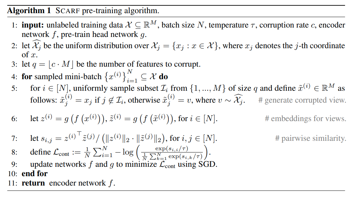
This paper tackles the problem of representation learning with tabular data. The paper proposes a framework called SCARF or Self-Supervised Contrastive Learning using Random Feature Corruption. There are 2 stages for this framework. The first stage is a self supervised stage where the create a corrupted view of a data instance using mask with some noise. The pass the instance and its perturbed view into an encoder and a projector to obtain final projects for the instance and its corrupted view. Then they calculate the InfoNCE to find out similarity between the instance and its corrupted view. The second stage is a supervised stage where they use the encoder from the first stage, removw the projector and add a predictor head to predict the class of the instance. They compared many noising schemes for the perturbation and found that swap noise, or replacing the values of the features with values from other instances, is the best.

Problem representation learning on tabular data

Solution, Ideas and Why generate a noisy version of the input sample, obtain the representation and projection of both the sample and the correpted to measure similarity. best noising is swap noise with feature values from other samples.

Images

Semantic-aware auto-encoders for self-supervised representation learning

BibTex
@inproceedings{wang2022semantic,
title={Semantic-aware auto-encoders for self-supervised representation learning},
author={Wang, Guangrun and Tang, Yansong and Lin, Liang and Torr, Philip HS},
booktitle={Proceedings of the IEEE/CVF Conference on Computer Vision and Pattern Recognition},
year={2022}}

url= https://openaccess.thecvf.com/content/CVPR2022/papers/Wang_Semantic-Aware_Auto-Encoders_for_Self-Supervised_Representation_Learning_CVPR_2022_paper.pdf
Summary

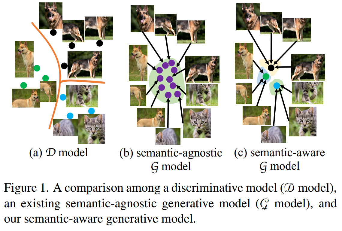
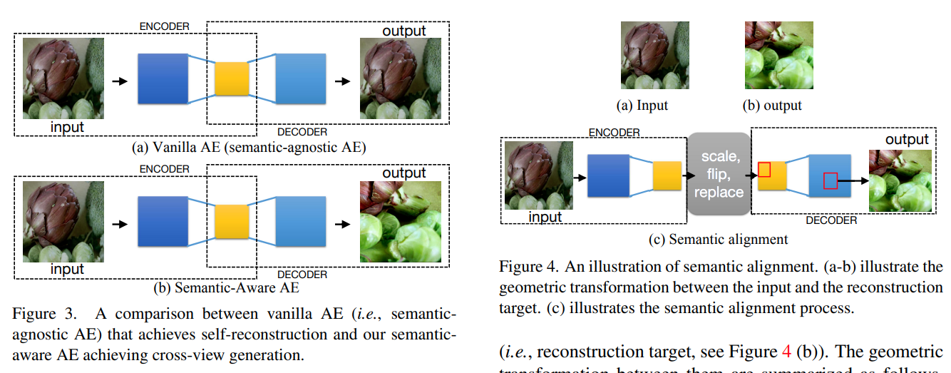
This paper tackles the problem of semantic aware generative feature learning. The authors noticed that previous approaches to self-supervised learning for images relied on discriminative models to learn features. They proposed a framework called Semantic-aware Auto-encoders for Self-supervised Representation Learning where they use a generative model to help learn the features. The framework works by generating two augmented views of the same sample. One view is passed to the encoder to obtain a representation. The representation is passed to the decoder to obtain to try to reconstruct the other view. Unfortunately, the decoder cannot guess the other view so they add transformations on the encoder feature maps (with spatial info) to align with the transformations on 2nd view, pass the transformed features maps to decoder to obtain reconstructed image, from which they obtain the final crop. They found that the transformations on the encoder feature maps are important for the decoder to learn. They also found That spatial information in feature maps for images are crucial and that global features that are not spatially aware are not good for reconstruction.

Problem generative representation learning

Solution, Ideas and Why learn semantic aware generative features by producing 2 augmented views, passing one the views to the encoder to get repr and pass the repr to decoder to get the other view. decoder cannot guess the target view so they add transformations on the encoder feature maps (with spatial info) to align with the transformations on 2nd view, pass the transformed features maps to decoder to obtain reconstructed image, from which they obtain the final crop

Images

On embeddings for numerical features in tabular deep learning

BibTex
@article{gorishniy2022embeddings,
title={On embeddings for numerical features in tabular deep learning},
author={Gorishniy, Yury and Rubachev, Ivan and Babenko, Artem},
journal={Advances in Neural Information Processing Systems},
year={2022}}

url= https://proceedings.neurips.cc/paper_files/paper/2022/file/9e9f0ffc3d836836ca96cbf8fe14b105-Paper-Conference.pdf
Summary

This paper tackles the problem of embedding numerical features in tabular data. The paper proposed a framework called Embeddings for Numerical Features in Tabular Deep Learning. This paper proposes two approaches for embedding numerical features in tabular data. The first approach is called Piecewise Linear Encoding (PLE) where the numerical features are binned and then each bin is encoded into a vector. Intuitively, the PLE reprsents how much the numerical value "fills" the embedding vector, where if the numerical value is greater than the bins, they are marked 1 in the target vector ("filled"), or the percentage of the bin filled if the value fell within the bin, or 0 otherwise. They discussed 2 approaches to find the bins. The first based on quantiles and the other on target aware bins obtained by a decision tree. The second approach is called Periodic Position Encoding (PPE) where the numerical features are encoded into a vector of sin and cosine of a source vector v with K learned coefficients of 2*pi*x where x is the numerical input. Intuitively, the PPE resembles a positional embedding for the value where K represent the embedding dimension (2K for sin and cosine), the range of the C values represents the number of cycles of 2 pi, the Cs represents offsets from zero of the numerical value, and x represents the multiplier of all C's to get the final value. Those Cs were learned and saved as constants to be used in inference.

Problem learning tabular data with numerical features

Solution, Ideas and Why Embed numerical feature values into vectors using piecewise linear encoding based on bins either quantile or target aware with a decision tree. Use periodic position encoding with concatenated vector of sin and cosine of a source vector v with K learned coefficients of 2*pi*x where x is the numerical input

VICReg: Variance-Invariance-Covariance Regularization for Self-Supervised Learning

BibTex
@inproceedings{bardes2021vicreg,
title={VICReg: Variance-Invariance-Covariance Regularization for Self-Supervised Learning},
author={Bardes, Adrien and Ponce, Jean and LeCun, Yann},
booktitle={International Conference on Learning Representations},
year={2021}}

url=https://openreview.net/pdf?id=xm6YD62D1Ub
Summary

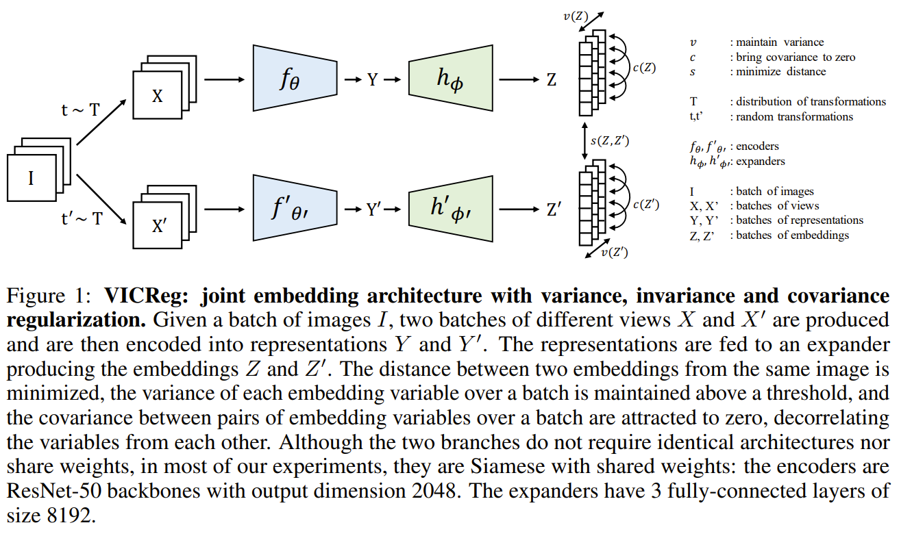
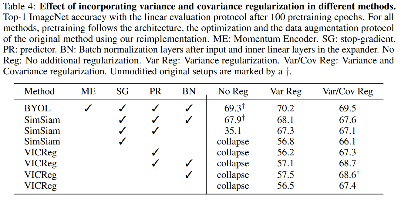
This paper tackles the problem of avoid collapse to a constant function in representation learning. The authors noticed that previous approaches to repreentation learning relied on negative samples, momentum encoders, or stop gradient to avoid collapse. They proposed a framework called VICReg or Variance-Invariance-Covariance Regularization for Self-Supervised Learning. The framework works by generating 2 augmented batches of views of the same input batch. The 2 batches are passed into an encoder and a projector to obtain 2 batches of projections. The first term in their loss is the invariance term which is the mean square distance between the 2 batches of projections. The invariance term serves to determine that the 2 batches of projections are similar since they are from the same batch of inputs samples. The second term is the variance term which is to prevent collapse to a constant functions. The variance term insures that the variance of the projections are above a threshold meaning that there is enough variety between the projections and thus the representations are not collapsed to a constant vector. The third term is the covariance term which is to prevent information collapse. The covariance term insures that features of the projections are not correlated, meaning that the features are not collapsed to a single feature. In their ablative studies, they found that their methods performs the best when all 3 term are used together with also batch normalization.

Problem avoid collapse without using negative pairs, momentum encoders, or stop gradient

Solution, Ideas and Why from a batch of images, a pair of augmented batches passed into encoder and projector to obtain batch of augmented projections. and an invariance term to measure the mean square distance between augmented views. The distance is to be minimized. Variance and Covariance Regularizer terms to respectively prevent collapse to a constant and information collapse (highly correlated features). Variance term insure variance of the projections are above threshold chosen, and Covariance insure uncorrelated features.

Images

Masked autoencoders are scalable vision learners

BibTex
@inproceedings{he2022mae,
title={Masked autoencoders are scalable vision learners},
author={He, Kaiming and Chen, Xinlei and Xie, Saining and Li, Yanghao and Doll{\'a}r, Piotr and Girshick, Ross},
booktitle={Proceedings of the IEEE/CVF conference on computer vision and pattern recognition},
year={2022}}

url= https://openaccess.thecvf.com/content/CVPR2022/papers/He_Masked_Autoencoders_Are_Scalable_Vision_Learners_CVPR_2022_paper.pdf
Summary

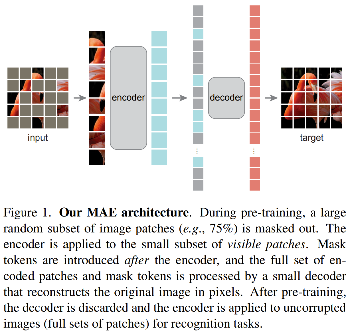
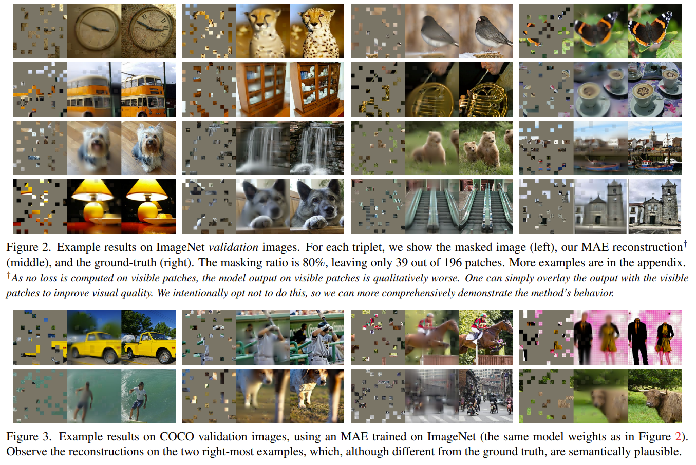
This paper tackles the problem of representation learning with masked image modeling. The authors noticed that masking an image with random 16x16 patches coveraging more than 75% of the image provides a difficult task for the encoder to learn a good semantic representation of the image without simply exploiting the spatial information locality in the image. They proposed a framework called Masked Autoencoders where they mask random 75% patches of the image using 16x16 patches and pass only the visible patches to the encoder (Vision Transformer) to obtain a representation. They then add mask tokens to the representation, which are indictive of the absence of visible patches in those areas. The representation with the mask tokens are passed to the decoder to predict the missing patches. The authors proposed an asymmetric auto encoder where the decoder is much smaller than the encoder to reduce compute cost. The decoder is then trained to predict only the missing patches. Through their experiments, they found that a high mask ratio offered a difficult task for the encoder to learn a good representation. They also found that passing only the visible patches reduced the computational cost of training a large encoder.

Problem generative representation learning with masked image modeling

Solution, Ideas and Why mask random 75% patches of image, pass only visible patches to encoder to get representation, add mask tokens to repr before passing to encoder to get pred missing patches asymmetric Auto Encoder where the decoder is much smaller than the encoder to reduce compute cost

Images

SimMIM: A simple framework for masked image modeling

BibTex
@inproceedings{xie2022simmim,
title={Simmim: A simple framework for masked image modeling},
author={Xie, Zhenda and Zhang, Zheng and Cao, Yue and Lin, Yutong and Bao, Jianmin and Yao, Zhuliang and Dai, Qi and Hu, Han},
booktitle={Proceedings of the IEEE/CVF Conference on Computer Vision and Pattern Recognition},
year={2022}}

url= https://openaccess.thecvf.com/content/CVPR2022/papers/Xie_SimMIM_A_Simple_Framework_for_Masked_Image_Modeling_CVPR_2022_paper.pdf
Summary

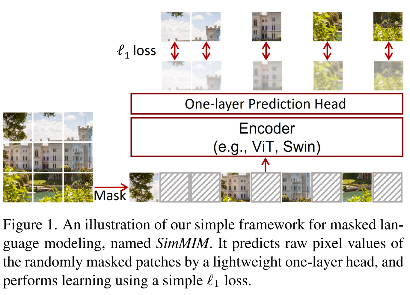
This paper tackles the problem of representation learning with masked image modeling. Similarly to MAE, the authors were using a Masked Autoencoder and masked significant portion of the image with random 32x32 mask patches. Unlike MAE, they passed both visible and mask patches to the encoder to obtain representations. Those representation vectors were passed to the decoder (without need to pass mask tokens) to predict the missing patches. They went smaller with the decoder and used a single linear layer to predict the missing patches. Their training objective was to predict raw pixel values for the missing patches.

Problem generative representation learning with masked image modeling

Solution, Ideas and Why mask random 60% 32x32 patches of image and pass both mased and visible patches to encoder to get representation and pass representation to 1 layer Linear decoder head to predict missing patches only at raw pixel level. learned mask token vectors are used to replace masked patches. The decoder is a small linear layer (asymmetric AE) and predicting raw pixel value works best

Images

SAINT: Improved neural networks for tabular data via row attention and contrastive pre-training

BibTex
@inproceedings{somepalli2022saint,
title={SAINT: Improved Neural Networks for Tabular Data via Row Attention and Contrastive Pre-Training},
author={Somepalli, Gowthami and Schwarzschild, Avi and Goldblum, Micah and Bruss, C Bayan and Goldstein, Tom},
booktitle={NeurIPS 2022 First Table Representation Workshop},
year={2022}}

url= https://openreview.net/pdf?id=FiyUTAy4sB8
Summary

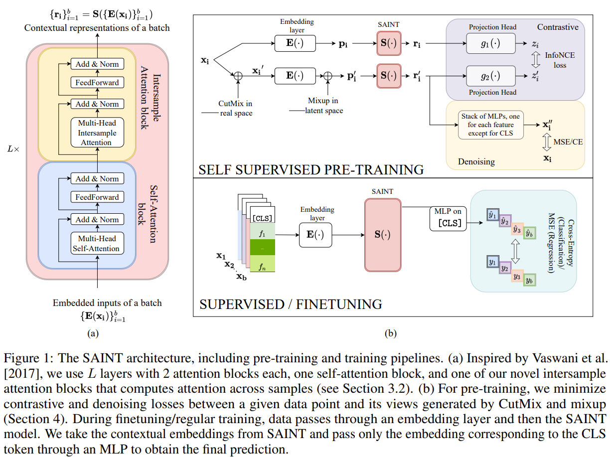
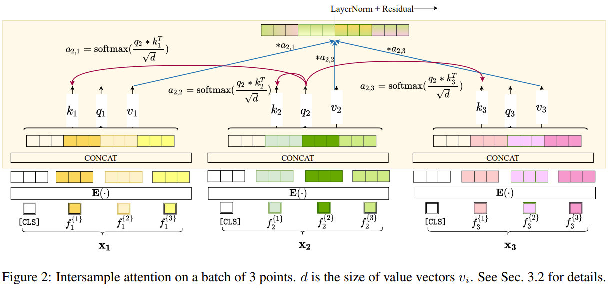
This paper tackles the problem of learning on tabular data. They noticed how deep learning methods still behind traditional methods on tabular data. They proposed a framework called SAINT or Self-Attention intersample attention transformer for tabular data. First they embed both categorical and numerical values in an embedding vector before passing it to their SAINT transformer. Their transformer uses 2 kinds of attention, self attention between features and their proposed intersample attention between rows. The intersample attention is calculated by computing the attention score between the query row and all other rows. that attention score dictates how much of the features of other samples will be used to produce the representation of the query row. They also proposed a 2 stage training where they first pretrain in a self supervised manner with contrastive loss between the projection of the row and its noisy augmented view, and with reconstructing the row from its noisy view projection. The second stage is a supervised finetuning stage for the downstream task. They used CutMix and MixUp for data corruption.

Problem learning tabular data

Solution, Ideas and Why intersample attention or attention across rows on top of self attention between columns (features). 2 stages, self supervised pretraining with contrative loss between projections of a sample and its noisy augmented view, and with reconstructing the sample from its noisy view reprresentation. Supervised finetuning stage follows.

Images

Self-supervised Learning is More Robust to Dataset Imbalance

BibTex
@inproceedings{liu2021rwsam,
title={Self-supervised Learning is More Robust to Dataset Imbalance},
author={Liu, Hong and HaoChen, Jeff Z and Gaidon, Adrien and Ma, Tengyu},
booktitle={International Conference on Learning Representations},
year={2021}}

url=https://openreview.net/pdf?id=4AZz9osqrar
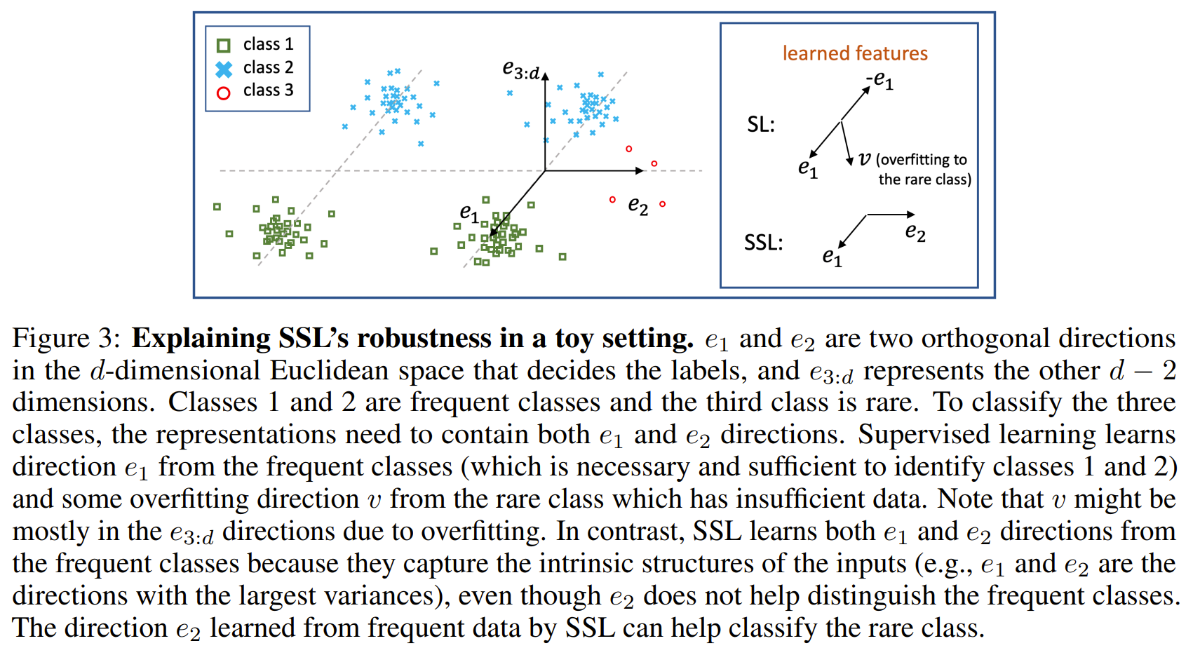
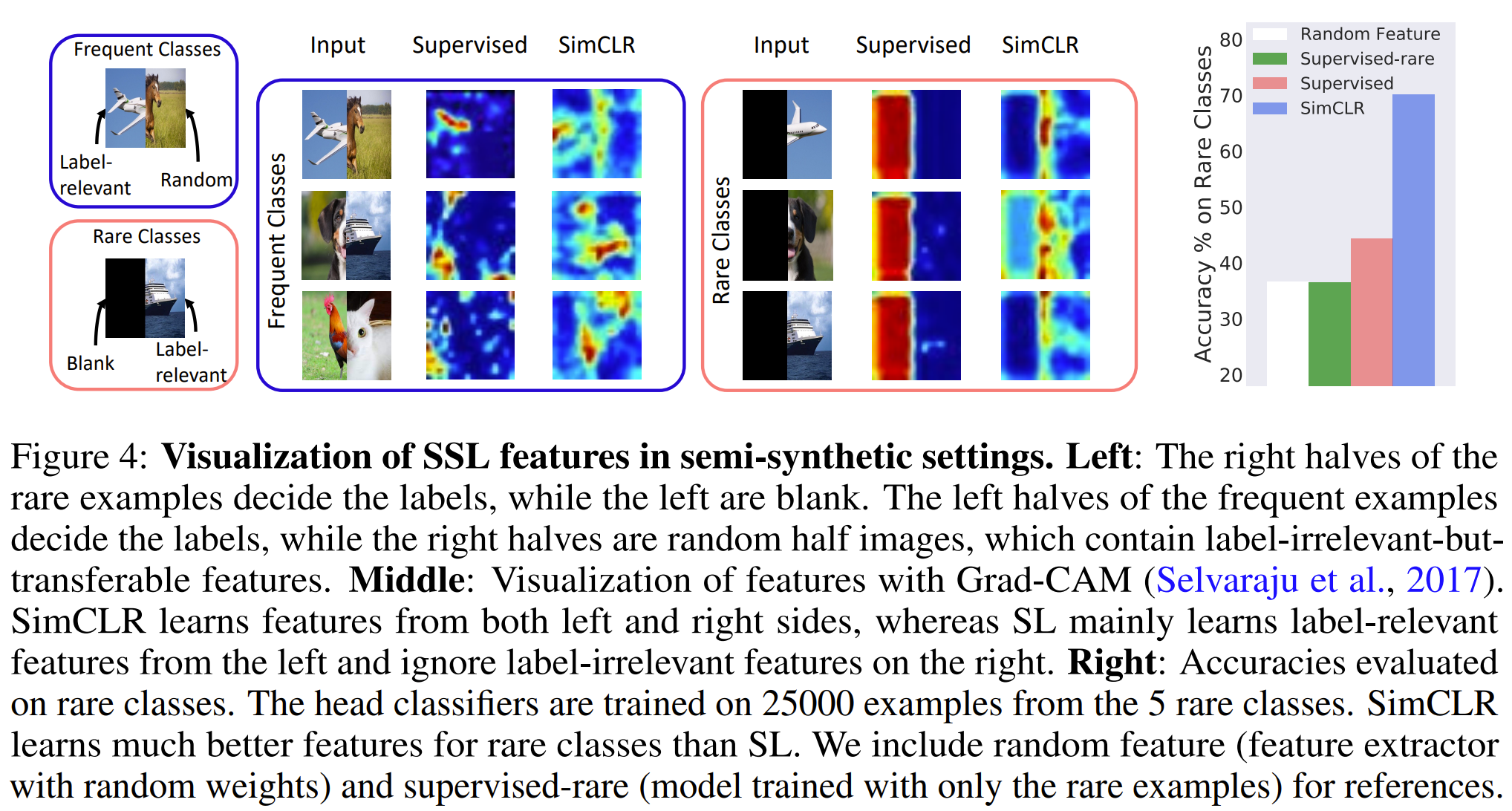
Summary

Investigated the robustness of SSL to imbalance in data and has better results on OoD cases. Without labels, net is less sensitive to outlier compared to with labels. SSL does this by learning the intrinsic structure of the input data. SL can overfit to noise if it is consistent enough. It's hard to rebalance without labels so instead we can use the loss sharpness where a sharper loss indicate harder and therefore tailer sample. Using KDE on the repr, they measure the loss in the neighborhood of the sample and if that loss is uniformly low, it's weight less and if it's uniformly high, it is weighted more.

Problem imbalance data in self supervised learning

Images

data2vec: A General Framework for Self-supervised Learning in Speech, Vision and Language,

BibTex
@inproceedings{baevski2022data2vec,
title={Data2vec: A general framework for self-supervised learning in speech, vision and language},
author={Baevski, Alexei and Hsu, Wei-Ning and Xu, Qiantong and Babu, Arun and Gu, Jiatao and Auli, Michael},
booktitle={International Conference on Machine Learning},
year={2022}},

url=https://proceedings.mlr.press/v162/baevski22a/baevski22a.pdf
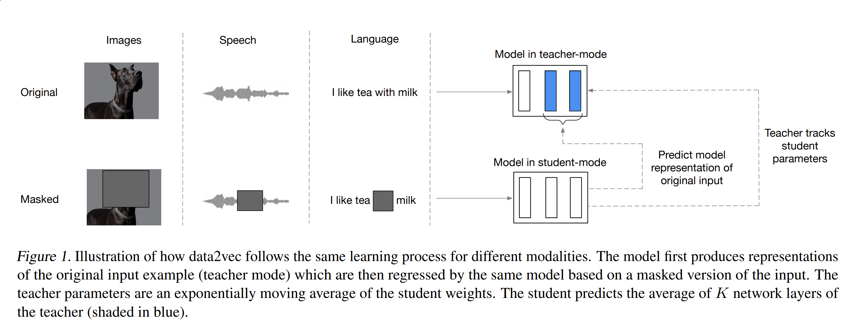
Summary

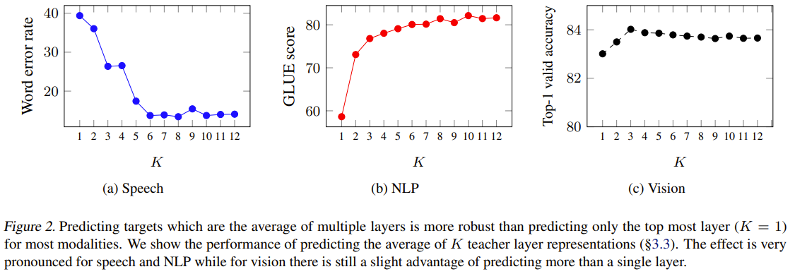
2 networks, ema teacher which takes original input (image or text or sound) to produce embeddings and a student which takes masked input to produce embeddings and predictions of the teacher avg of K layers outputs. Their objective is smooth L1 loss which transition from square loss to l1 loss when the error of a particular sample is greater than a threshold beta. The equations are setup with additional terms of beta to transition the function smoothly. This help mitigate outliers.

Problem predict embedding

Images

Masked Siamese Networks for Label-Efficient Learning

BibTex
@inproceedings{assran2022msn,
title={Masked siamese networks for label-efficient learning},
author={Assran, Mahmoud and Caron, Mathilde and Misra, Ishan and Bojanowski, Piotr and Bordes, Florian and Vincent, Pascal and Joulin, Armand and Rabbat, Mike and Ballas, Nicolas},
booktitle={European Conference on Computer Vision},
year={2022}}

url=https://www.ecva.net/papers/eccv_2022/papers_ECCV/papers/136910442.pdf
Summary

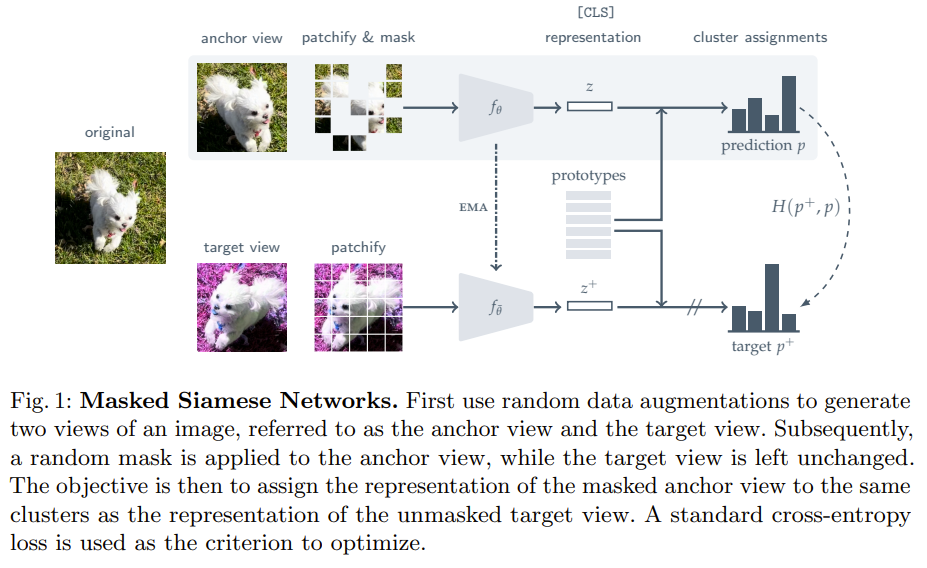
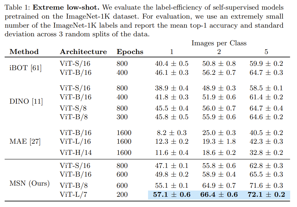
2 branches, anchor (online) branch and a ema (target) branch. Anchor branch get patchified and masked anchor image while target branch used augmentation and patchify target image. With learned cluster center (Dense), the objetive was to match cluster assignment from online to target branch To ensure the clusters formed are roughly the same size (same number of elements), they explicitly maximize the mean entropy of the assignment prediction. The max entropy is when their probabilities are the same and they are uniformly distributed

Problem predict embedding

Images

The hidden uniform cluster prior in self-supervised learning

BibTex
@inproceedings{assran2022hidden,
title={The hidden uniform cluster prior in self-supervised learning},
author={Assran, Mido and Balestriero, Randall and Duval, Quentin and Bordes, Florian and Misra, Ishan and Bojanowski, Piotr and Vincent, Pascal and Rabbat, Michael and Ballas, Nicolas},
booktitle={The Eleventh International Conference on Learning Representations},
year={2022}}

url=https://openreview.net/pdf?id=04K3PMtMckp
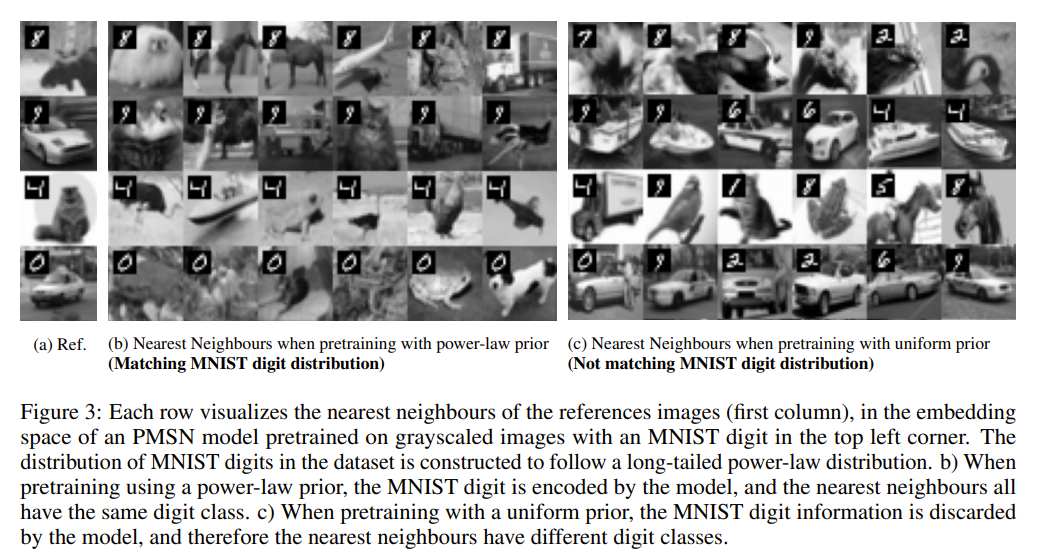
Summary

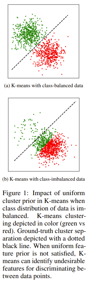
Contrastive Methods can be showed to reduce to implicit or explicit k-means clustering. those can be further divided into instance based or volume maximizing. Volume maximi- zing does worse on imbalance because they assume clusters are of equal size The hidden cluster prior is addressed by explicit incentivizing the clusters formed to be less uniform and more like a pareto distribution. Assume the distribution of the data is known and can be provided to the algorithm

Problem imbalanced data

Images

Divide and contrast: Self-supervised learning from uncurated data

BibTex
@inproceedings{tian2021dnc,
title={Divide and contrast: Self-supervised learning from uncurated data},
author={Tian, Yonglong and Henaff, Olivier J and van den Oord, A{\"a}ron},
booktitle={Proceedings of the IEEE/CVF International Conference on Computer Vision},
year={2021}}

url=https://openaccess.thecvf.com/content/ICCV2021/papers/Tian_Divide_and_Contrast_Self-Supervised_Learning_From_Uncurated_Data_ICCV_2021_paper.pdf
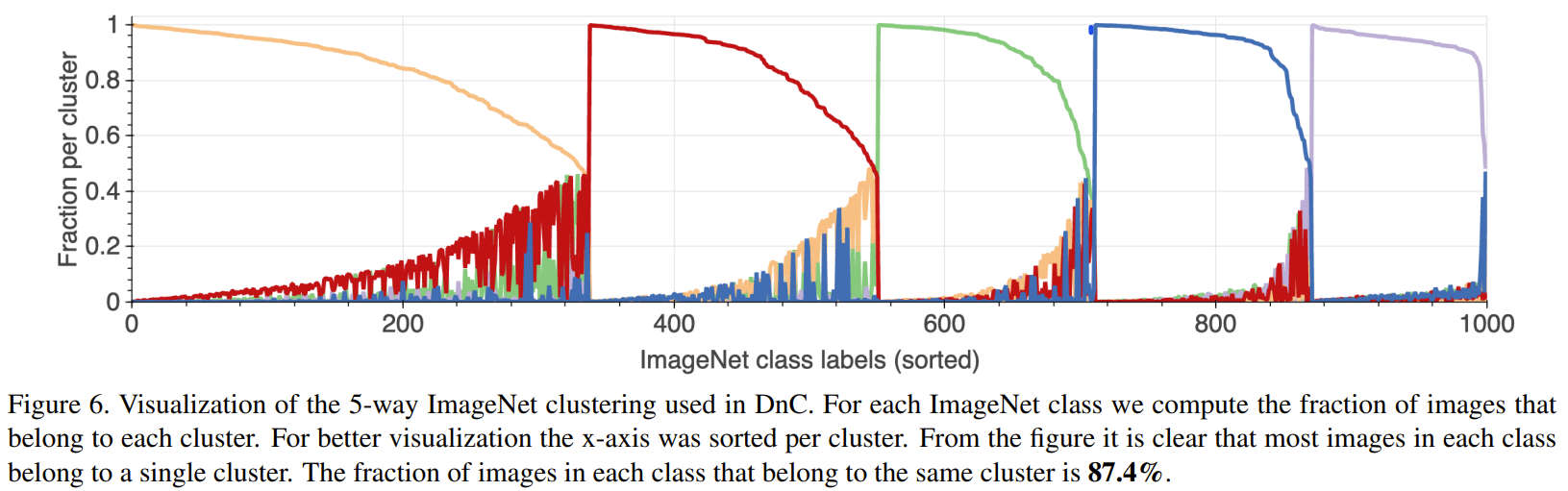
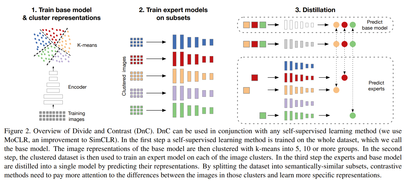
Summary

train base model on uncurated data to using CL to get repr that will be clustered using k-means. Original dataset is split according to the cluster and expert models are trained on individual subsets using CL. For any sample, the base model and the appropriate expert is used to distill knowledge into student. The student model learns to predict the project of the teachers models with its additional regression head. The subsets allow for hard negative mining which incentivizes learning better expert representations. Base model helps tie repr space together.

Problem imbalanced uncurated data

Images

Improving contrastive learning on imbalanced data via open-world sampling

BibTex
@article{jiang2021mak,
title={Improving contrastive learning on imbalanced data via open-world sampling},
author={Jiang, Ziyu and Chen, Tianlong and Chen, Ting and Wang, Zhangyang},
journal={Advances in Neural Information Processing Systems},
year={2021}}

url=https://proceedings.neurips.cc/paper_files/paper/2021/file/2f37d10131f2a483a8dd005b3d14b0d9-Paper.pdf
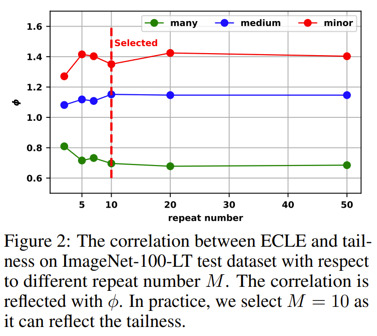
Summary

compensate for imbalance in data by sampling external data according to tailness, proximity, diversity. Tailness where the hard samples according to ECLE are considered tail, diversity to prevent similar samples, and proximity to prevent OoD outlier samples ECLE is based on expected contrastive loss over many augmentations for the views to smooth out the randomness of augmentations so the ECLE is only attributed to tailness. When applying K-center greedy, they use min because min garantees that the sample will be further away than any other.

Problem imbalanced data

Images

Representation learning with contrastive predictive coding

BibTex
@article{oord2019cpc,
title={Representation learning with contrastive predictive coding},
author={Oord, Aaron van den and Li, Yazhe and Vinyals, Oriol},
journal={arXiv preprint arXiv:1807.03748},
year={2019}}

url=https://arxiv.org/pdf/1807.03748.pdf
Summary

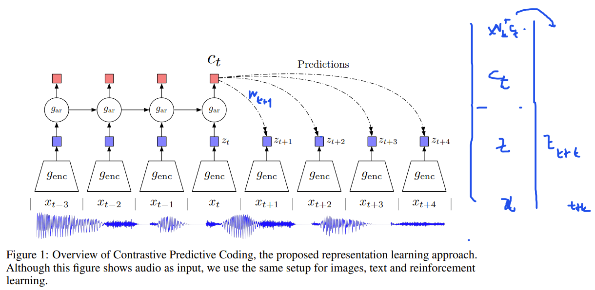
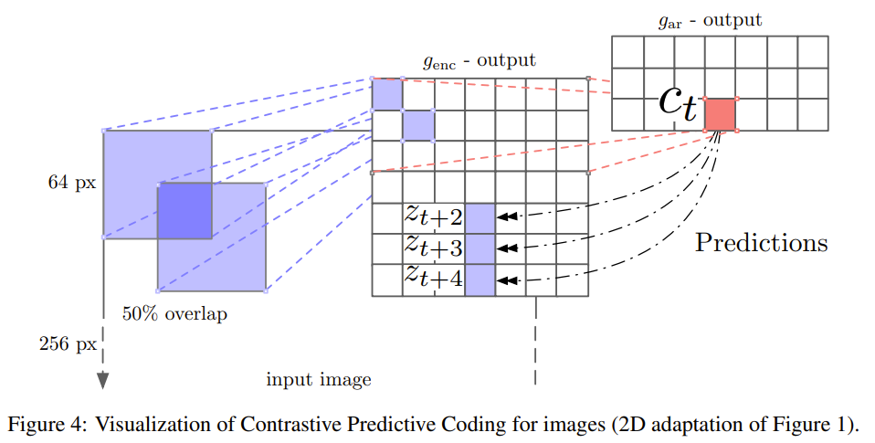
from time series, use encoder to produce timestep representation z and use an autoregressive encoder to produce representation context c across timesteps. Context of repr in the past is used to predict the repr z of future timesteps using CL where a positve pair is with Wc and z in the future. from time series, use encoder to produce timestep representation z and use an autoregressive encoder to produce representation context c across timesteps. Context of repr in the past is used to predict the repr z of future timesteps using CL where a positve pair is with Wc and z in the future

Problem time series data

Images

Unsupervised scalable representation learning for multivariate time series

BibTex
@article{franceschi2019tloss,
title={Unsupervised scalable representation learning for multivariate time series},
author={Franceschi, Jean-Yves and Dieuleveut, Aymeric and Jaggi, Martin},
journal={Advances in neural information processing systems},
year={2019}}

url=https://proceedings.neurips.cc/paper/2019/file/53c6de78244e9f528eb3e1cda69699bb-Paper.pdf
Summary

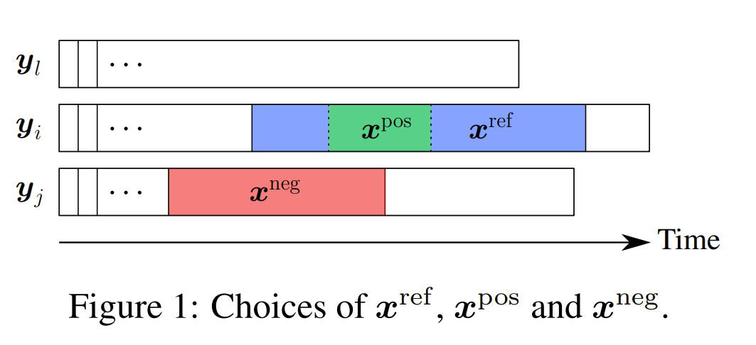
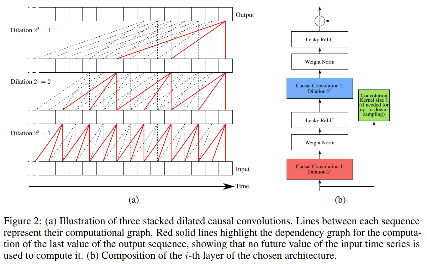
using triplet loss where a reference subseries is taken from a batch of series, a positive subseries taken from the reference subseries to form a positive pair with the reference. K negative subseries are taken from any other series in the batch to form a negative pair. dilated convolution where the stride and the filter size is the same for every layer but the dilation increase by factor of 2 at every layer, increasing the distance between 2 consecutive weights. To handle multivariate series, the increase the dimensionality of the filters from 1 to 2 where the added dim is for the additional vars

Problem time series data

Images

Unsupervised Representation Learning for Time Series with Temporal Neighborhood Coding

BibTex
@inproceedings{tonekaboni2020tnc,
title={Unsupervised Representation Learning for Time Series with Temporal Neighborhood Coding},
author={Tonekaboni, Sana and Eytan, Danny and Goldenberg, Anna},
booktitle={International Conference on Learning Representations},
year={2020}}

url=https://openreview.net/pdf?id=8qDwejCuCN
Summary

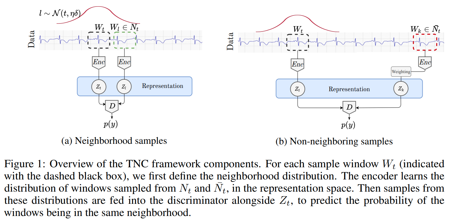
define a time window Wt centered at a reference timestep t of width delta. From Wt, define a a temporal neighborhood as a gaussion distribution over the time windows with mean Wt and variance defined by eta*delta. Given the anchor window Wt and the temp neighborhood of Wt, a positive sample is one from the neighborhood and a "negative" sample is one outside the hood Sampling bias in MTS where even outsdie of the hood, a sample window can still have similarities with the anchor window. To tackle this, consider outside neighborhood as unlabeled with some prob w to be positive (similar) and 1-w to be (dissimilar). They use a Disciminator Net with BCE with output 1 as 2 repr of windows in hood and 0 outside the hood.

Problem representation learning on time series

Images

A Transformer-based Framework for Multivariate Time Series Representation Learning

BibTex
@inproceedings{zerveas2021tst,
title={A transformer-based framework for multivariate time series representation learning},
author={Zerveas, George and Jayaraman, Srideepika and Patel, Dhaval and Bhamidipaty, Anuradha and Eickhoff, Carsten},
booktitle={Proceedings of the 27th ACM SIGKDD conference on knowledge discovery \& data mining},
year={2021}}

url=https://dl.acm.org/doi/pdf/10.1145/3447548.3467401
Summary

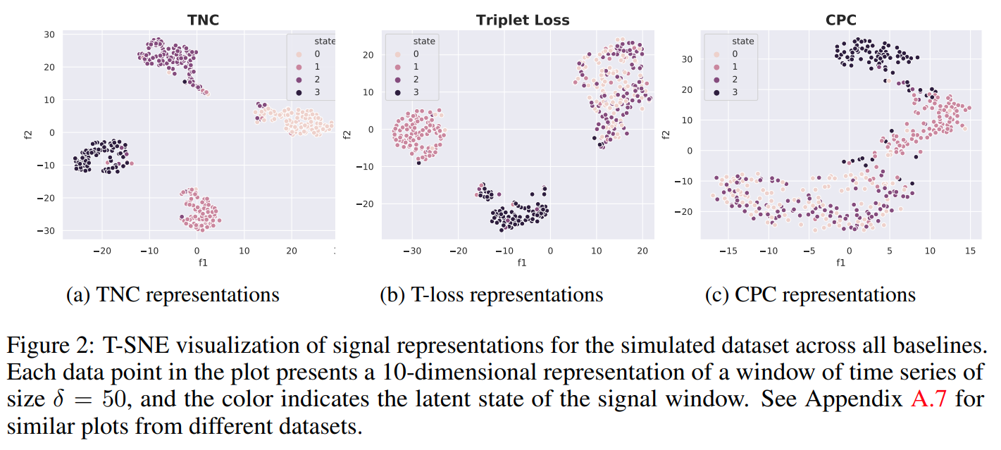
From MTS, input variable vector at time t is encoded with a Linear layer into d dimensional vector. to further reduce the resolution in time of the MTS, a 1D conv can be applied to summary multiple timesteps into 1. Once d dim vector is obtained, learned positional embedding are added to produce the final input for encoder only transformer. The encoder is then used to produce representation per timesteps. They trained first with unsupervised where a fraction of the input window was masked and the network predicts the mask input to reconstructed the window. They then trained for the downstream task where for a window, they obtain representations for each timesteps and concatenate them into the full window representation.

Problem using transformer for time series data

Images

Time-series representation learning via temporal and contextual contrasting

BibTex
@article{eldele2021tstcc,
title={Time-series representation learning via temporal and contextual contrasting},
author={Eldele, Emadeldeen and Ragab, Mohamed and Chen, Zhenghua and Wu, Min and Kwoh, Chee Keong and Li, Xiaoli and Guan, Cuntai},
journal={Proceedings of the Thirtieth International Joint Conference on Artificial Intelligence (IJCAI-21)},
year={2021}}

url=https://www.ijcai.org/proceedings/2021/0324.pdf
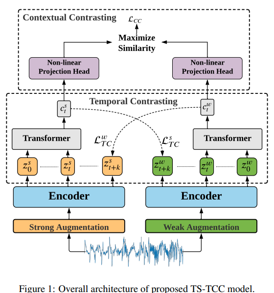
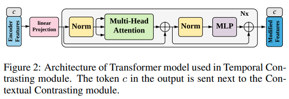
Summary

From a time series, they produce 2 augs, a weak aug (jitter and scale) and a strong aug (segment suffling and jitter). From the 2 augs from the same sample, they are encoded into repr per timesteps. they do temporal contrating where the repr are used to produce context summarizing past timesteps. From context of an aug, they predict the future repr of the other aug as positive pair. neg pair are other sample repr in minibatch. They also do contextual repr where from the context of both augs, they measure the cosine similarity and that similarity should be maximized for contexts of augs from the same sample and minimized for contexts of augs from different samples. During experimentation, they found contextual contrastive is of higher importance than temporal contrasting

Problem time series representation

Images

Ts2vec: Towards universal representation of time series

BibTex
@inproceedings{yue2022ts2vec,
title={Ts2vec: Towards universal representation of time series},
author={Yue, Zhihan and Wang, Yujing and Duan, Juanyong and Yang, Tianmeng and Huang, Congrui and Tong, Yunhai and Xu, Bixiong},
booktitle={Proceedings of the AAAI Conference on Artificial Intelligence},
year={2022}}

url=https://ojs.aaai.org/index.php/AAAI/article/view/20881/20640
Summary

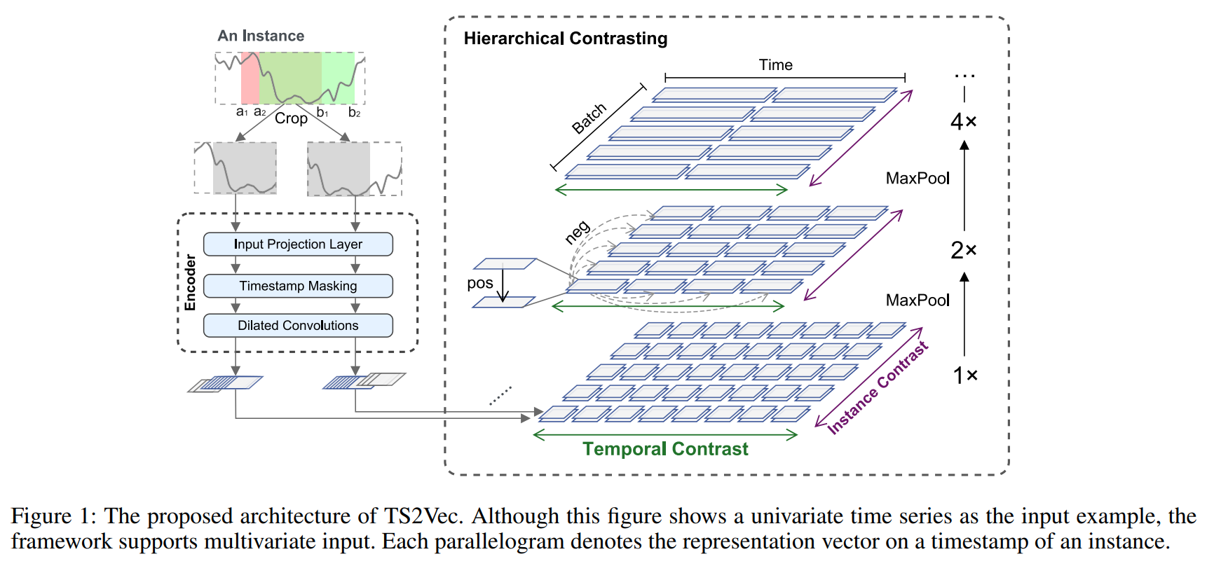
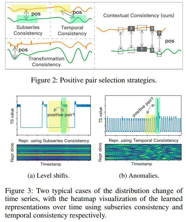
from a time series, they produce 2 augs which are random croppings with an overlapping region to incentivize contextual consistancy between the augs. Cropping doesn't affect the amplitude of the series. From the 2 crops, the obtain per timestep projections. In the overlapping region, they mask random timesteps according to bernoulli distribution in such a way that they are visible in the second aug if masked in the first and vice versa. From masked views they obtain repr using Dialated conv. they employ hierarchical contrasting composed of temporal and instance-wise contrasting summed at multiple semantic levels using maxpooling (dividing the repr series in half) to incentivize temporal invariance of the representations. The temporal contrasting is considering a view of a sample at a time t and the other view of the sample at the same time t as positive pair, while all other timesteps of both views for the same sample are negative. The instance-wise contrasting considers the repr of the views from the same sample at the same timestep as positive pair while the reprs of the views of other instances at the same timestep are negative.

Problem time series representations

Images

Dynamic sparse network for time series classification: Learning what to “see”

BibTex
@article{xiao2022dns,
title={Dynamic sparse network for time series classification: Learning what to “see”},
author={Xiao, Qiao and Wu, Boqian and Zhang, Yu and Liu, Shiwei and Pechenizkiy, Mykola and Mocanu, Elena and Mocanu, Decebal Constantin},
journal={Advances in Neural Information Processing Systems},
year={2022}}

url=https://proceedings.neurips.cc/paper_files/paper/2022/file/6b055b95d689b1f704d8f92191cdb788-Paper-Conference.pdf
Summary

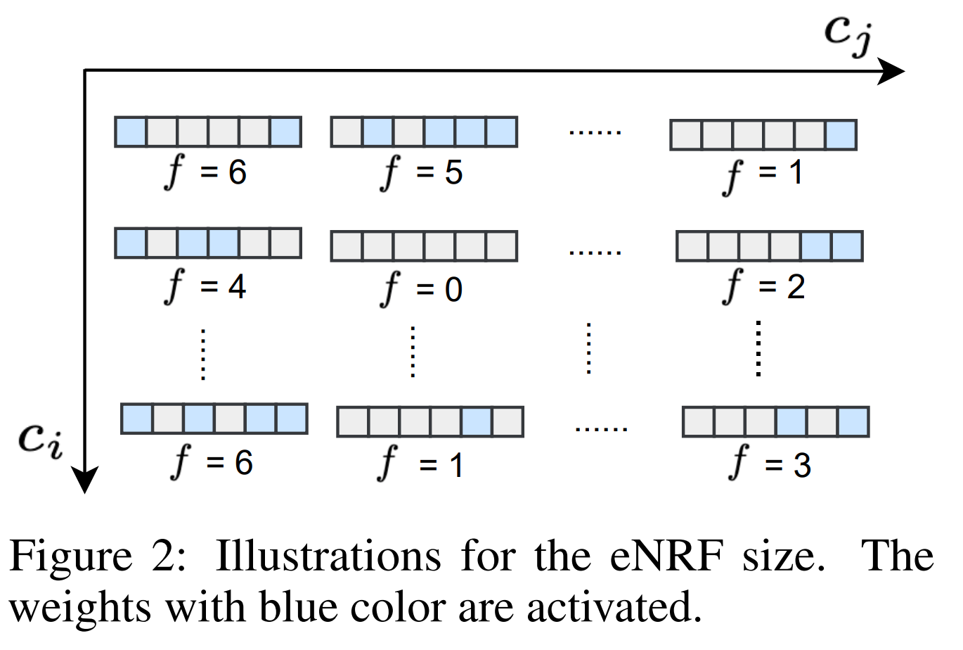
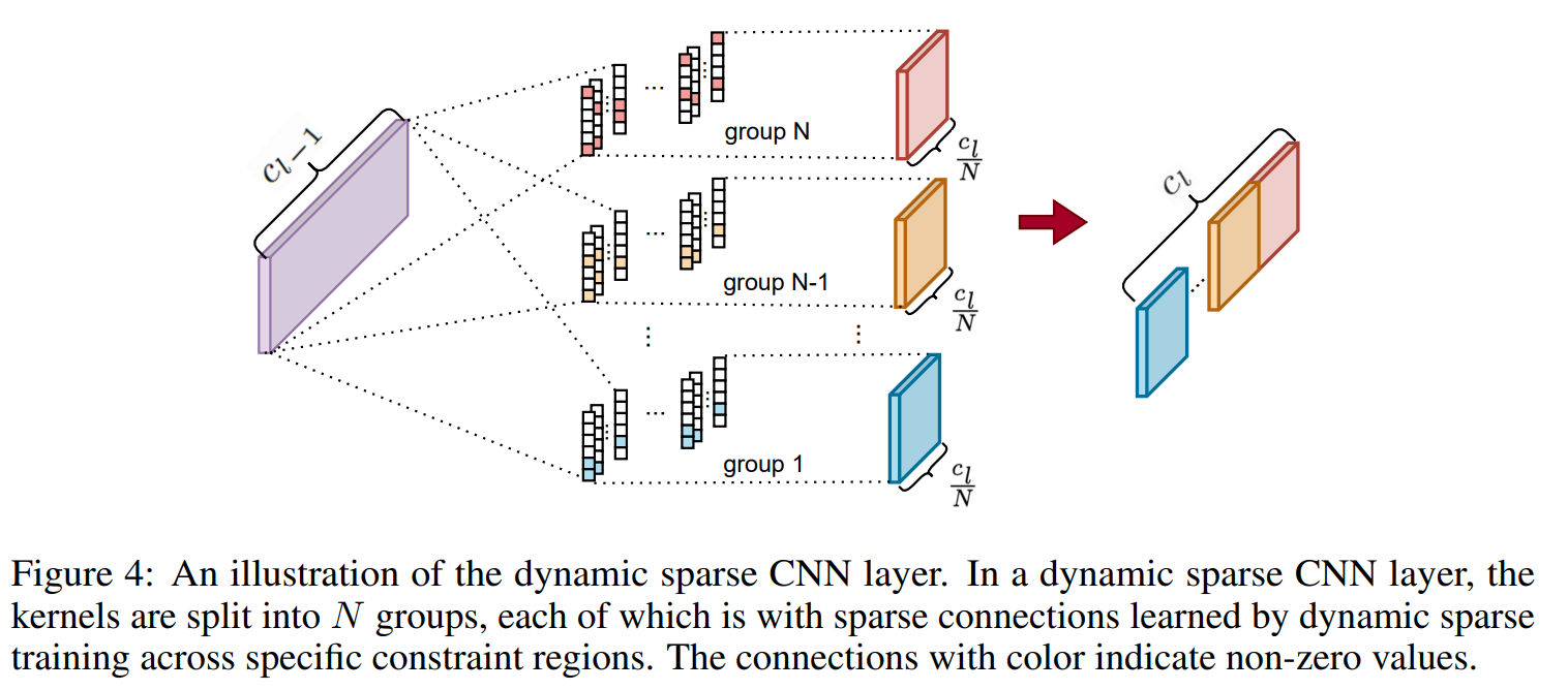
Use large sparse kernel that are dynamically "indicated" with a dynamic indicator function. the eNRF or effective neighborhood Receptive Field is the distance between the first and the last activate weight in the kernel layer. The indicator funtion is updated every set of epochs to insure the sparsity of the kernels. The kernels in each dynamic sparse layer are divided into groups corresponding to exploration regions for the kernel weights. Activated weights for a particular group are limited to the exploration region. This allows for various eNRF to be covered without biasing toward large receptive fields, and the exploration space to be reduced

Problem efficient representation of time series data

Images

Self-supervised contrastive pre-training for time series via time-frequency consistency

BibTex
@article{zhang2022tfc,
title={Self-supervised contrastive pre-training for time series via time-frequency consistency},
author={Zhang, Xiang and Zhao, Ziyuan and Tsiligkaridis, Theodoros and Zitnik, Marinka},
journal={Advances in Neural Information Processing Systems},
year={2022}}

url=https://proceedings.neurips.cc/paper_files/paper/2022/file/194b8dac525581c346e30a2cebe9a369-Paper-Conference.pdf
Summary

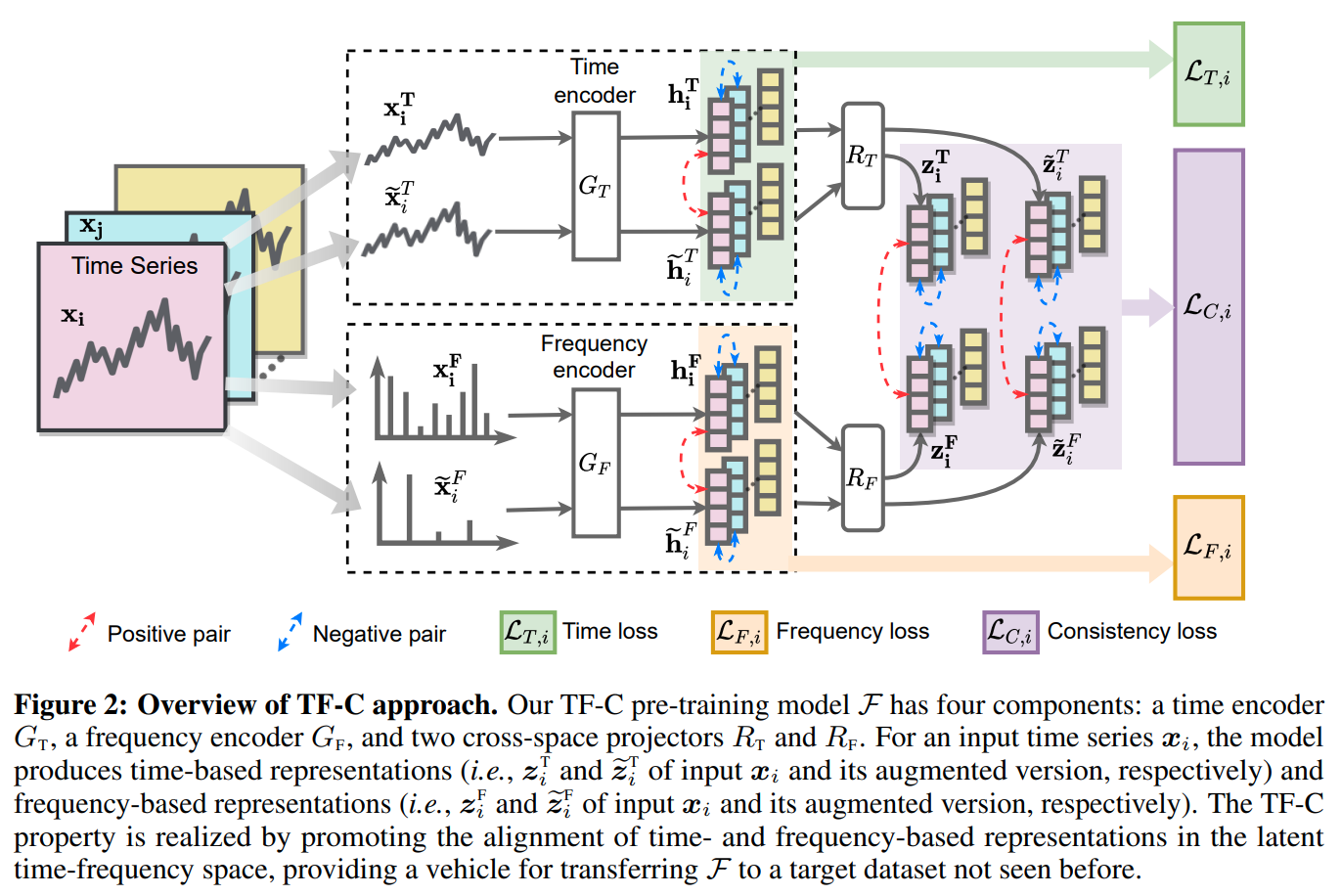
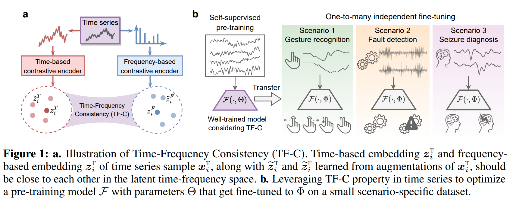
time-frequency consistency where from sample, the time based and frequency representation should be close. In addition to time based and freq based represenations, they produce repr of augmented views of both time based and freq based. In time-freq, reprs of the same sample in time and freq should be closer to each other than to repr of aug view in time and freq fo the same sample which should closer than to repr of other samples. in time, anchor view with aug view of the same sample is positive pair while anchor view with other samples and their views as negative pairs. Similarly in frequency. Their architecture has 4 networks. 2 encoder networks. Time enoder, a space encoder. 2 projectors, a time to time-space project and a freq to freq-time projector.

Problem representation learning of time series data

Images

CLOCS: Contrastive Learning of Cardiac Signals Across Space, Time, and Patients.

BibTex
@inproceedings{kiyasseh2021clocs,
title={Clocs: Contrastive learning of cardiac signals across space, time, and patients},
author={Kiyasseh, Dani and Zhu, Tingting and Clifton, David A},
booktitle={International Conference on Machine Learning},
year={2021}}

url=http://proceedings.mlr.press/v139/kiyasseh21a/kiyasseh21a.pdf
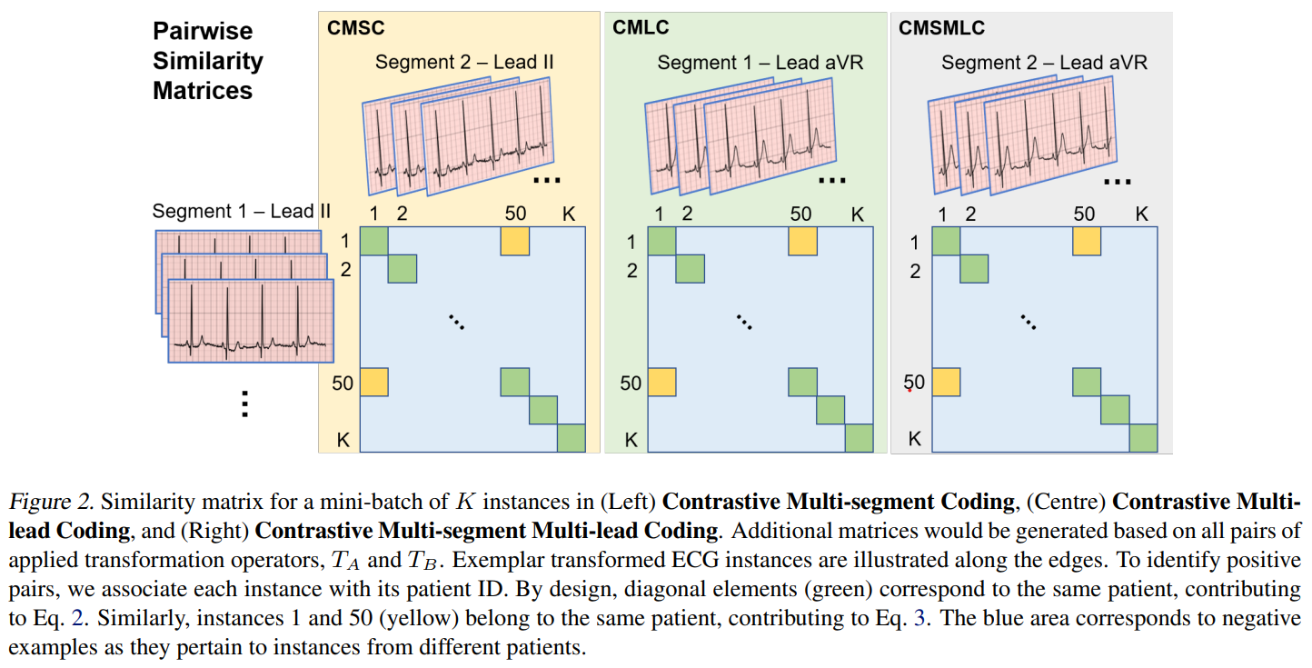
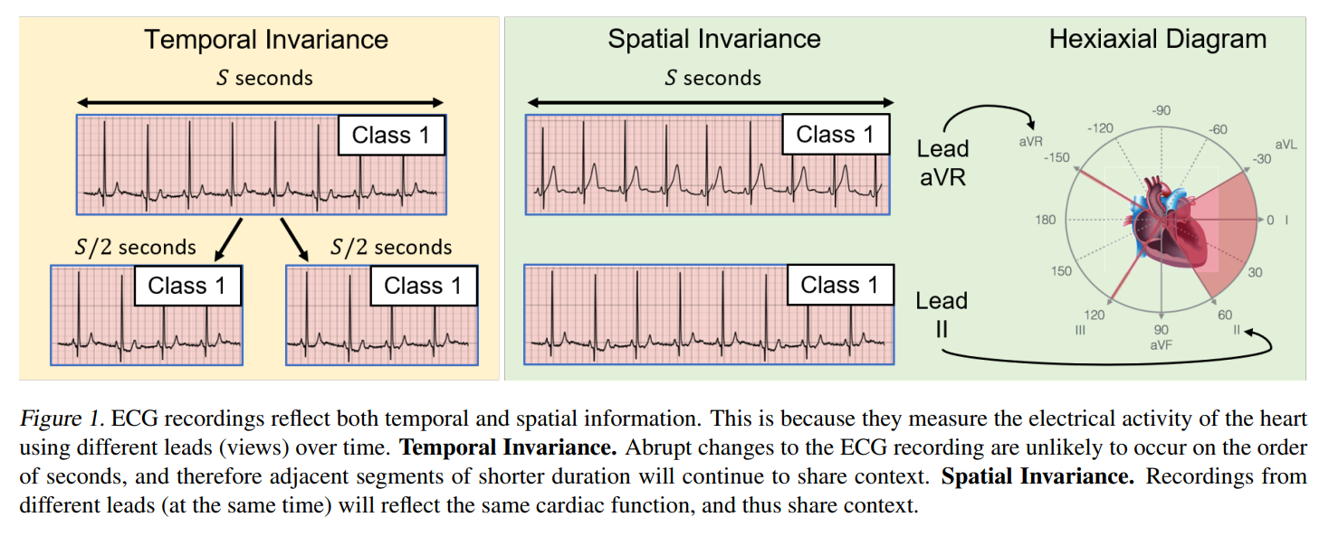
Summary

From samples they generate 2 sets augmented views. In addition they generate segments from the same samples (temporal consistency) and use different lead (spatial consistency) as augmented views. They measure the cosine similary and, when from different segments, different leads, diff segment and lead, or diff augmentatios, two view from the same patient (whether same or different instance sample) are positive and 2 view from different patients are negative. the transformation applied to the two view are flipped to make sure that the initial asymmetric contrastive learning equations 2 and 3 are symmetrized in equation 4.

Problem sample efficient time series representation learning

Images

CoST: Contrastive Learning of Disentangled Seasonal-Trend Representations for Time Series Forecasting

BibTex
@inproceedings{woo2021cost,
title={CoST: Contrastive Learning of Disentangled Seasonal-Trend Representations for Time Series Forecasting},
author={Woo, Gerald and Liu, Chenghao and Sahoo, Doyen and Kumar, Akshat and Hoi, Steven},
booktitle={International Conference on Learning Representations},
year={2021}}

url=https://openreview.net/pdf?id=PilZY3omXV2
Summary

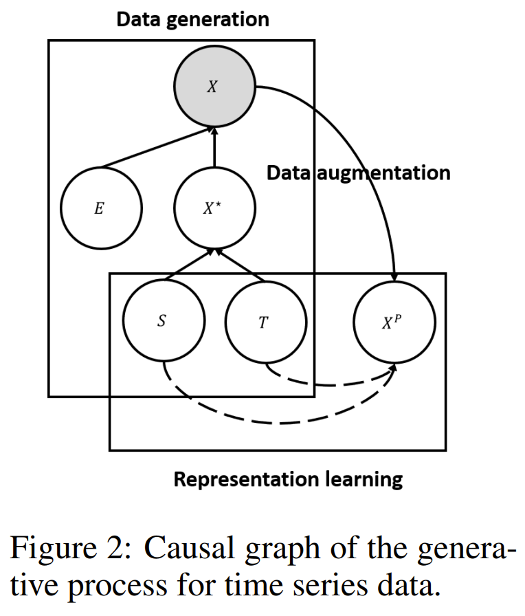
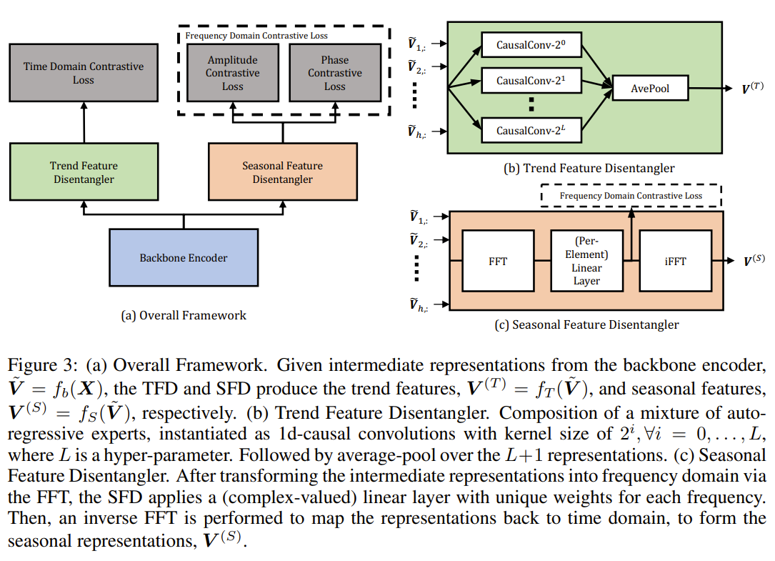
The authors propose CoST, a contrastive learning framework for learning disentangled seasonal-trend representations for time series forecasting. The key ideas and technical details are as follows: 1. Structural time series formulation: CoST assumes that the observed time series data X is generated from an error variable E and an error-free latent variable X*, which in turn is generated from a trend variable T and a seasonal variable S. The goal is to learn representations of T and S, which are invariant under changes in E, to achieve optimal prediction. 2. Contrastive learning: CoST uses data augmentations as interventions on the error variable E and learns invariant representations of T and S via contrastive learning. The contrastive loss encourages the model to learn representations that are invariant to the interventions on E. 3. Trend Feature Disentangler (TFD): The TFD extracts trend representations using a mixture of auto-regressive experts, which adaptively selects the appropriate lookback window. Each expert is implemented as a 1D causal convolution with a different kernel size. The outputs of the experts are averaged to obtain the final trend representations. The TFD is learned using a time-domain contrastive loss. 4. Seasonal Feature Disentangler (SFD): The SFD extracts seasonal representations using a learnable Fourier layer, which enables intra-frequency interactions. The intermediate representations are transformed into the frequency domain using the discrete Fourier transform (DFT). A learnable Fourier layer, implemented as a per-element linear layer with unique weights for each frequency, is applied to the frequency-domain representations. An inverse DFT is then performed to map the representations back to the time domain, forming the seasonal representations. 5. Frequency-domain contrastive loss: The SFD is learned using a frequency-domain contrastive loss, which consists of an amplitude component and a phase component. The loss encourages the model to learn discriminative seasonal representations without prior knowledge of the periodicity. 6. Training: CoST is trained end-to-end using a combined loss function that includes the time-domain contrastive loss for the TFD and the frequency-domain contrastive loss for the SFD. The outputs of the TFD and SFD are concatenated to form the final output representations. 7. Downstream forecasting: After training, the learned representations are used as input to a simple regression model, such as ridge regression, to perform time series forecasting. CoST achieves state-of-the-art performance on various real-world benchmark datasets, outperforming both end-to-end supervised forecasting methods and other representation learning approaches. The disentangled seasonal-trend representations learned by CoST are more robust to noise and distribution shifts, leading to improved generalization in non-stationary environments.

Problem Deep learning methods for time series forecasting often suffer from poor performance due to learning entangled representations from observed data, which may contain noise. This leads to the model capturing spurious correlations that do not generalize well, especially in non-stationary environments.

Images

Rank-N-Contrast: Learning Continuous Representations for Regression

BibTex
@article{zha2023RNC,
title={Rank-N-Contrast: Learning Continuous Representations for Regression},
author={Zha, Kaiwen and Cao, Peng and Son, Jeany and Yang, Yuzhe and Katabi, Dina},
journal={Advances in Neural Information Processing Systems},
year={2023}}

url= https://proceedings.neurips.cc/paper_files/paper/2023/file/39e9c5913c970e3e49c2df629daff636-Paper-Conference.pdf
Summary

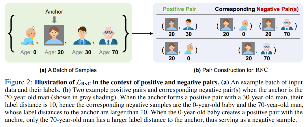
The authors propose Rank-N-Contrast (RNC), a framework that learns continuous representations for regression by contrasting samples against each other based on their rankings in the target space. The key ideas and technical details of RNC are as follows: 1. RNC introduces the LRNC loss, which first ranks the samples in a batch according to their labels and then contrasts them against each other based on their relative rankings. For each anchor sample, the likelihood of any other sample to be similar to the anchor increases exponentially with respect to their similarity in the representation space. The denominator of the likelihood is a sum over the samples that possess higher ranks than the current sample in terms of label distance to the anchor. 2. LRNC can be interpreted in the context of positive and negative pairs in contrastive learning. In regression, any two samples can be considered as a positive or negative pair depending on the context. For a given anchor sample, any other sample in the batch can be used to construct a positive pair, with the corresponding negative samples being all samples whose labels differ from the anchor's label by more than the label of the positive sample. 3. The authors prove that optimizing LRNC results in an ordered feature embedding that corresponds to the ordering of the labels. They introduce the concept of δ-ordered feature embeddings and show that as the optimization of LRNC approaches its lower bound, the feature embeddings become δ-ordered. The authors also provide an analysis based on Rademacher Complexity to prove that a δ-ordered feature embedding results in a better generalization bound. 4. RNC first learns a regression-aware representation using the LRNC loss and then leverages it to predict the continuous targets. The framework is compatible with existing regression methods, allowing for the use of any regression method to map the learned representation to the final prediction values. 5. The authors conduct ablation studies to investigate the impact of various components of RNC, such as the number of positive samples, the feature similarity measure, and the training scheme. The results show that considering all samples as positive, using negative L1 or L2 norm as the similarity measure, and employing the linear probing training scheme lead to the best performance. RNC provides a simple and effective approach to learn continuous representations for regression tasks, addressing the limitations of existing regression and representation learning methods. The learned representations capture the intrinsic ordered relationships between samples, leading to improved performance, robustness, and generalization in various real-world regression problems.

Problem Deep regression models often fail to capture the continuous nature of sample orders in the learned representations, leading to suboptimal performance across a wide range of regression tasks. Existing representation learning methods also overlook the intrinsic continuity in data for regression.

Images

Improving Deep Regression with Ordinal Entropy

BibTex
@inproceedings{zhang2022improving,
title={Improving Deep Regression with Ordinal Entropy},
author={Zhang, Shihao and Yang, Linlin and Mi, Michael Bi and Zheng, Xiaoxu and Yao, Angela},
booktitle={The Eleventh International Conference on Learning Representations},
year={2022}}

url=https://openreview.net/pdf?id=raU07GpP0P
Summary

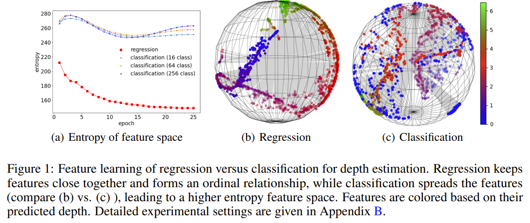
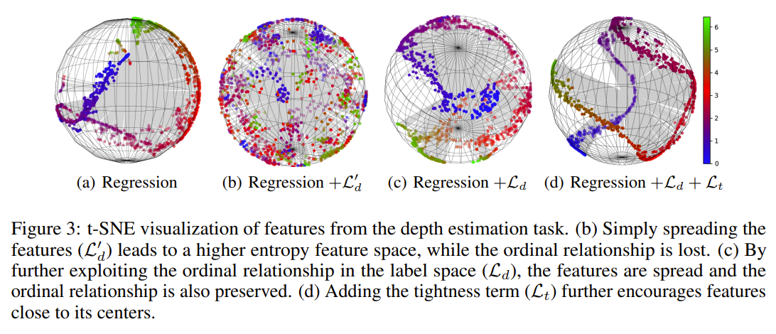
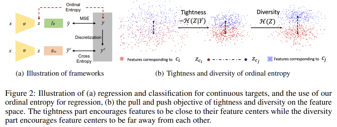
The authors propose an ordinal entropy regularizer to encourage higher-entropy feature spaces while maintaining ordinal relationships in regression tasks. The key ideas and technical details of the method are as follows: Mutual information analysis: The authors analyze the difference in feature learning between classification and regression from a mutual information perspective. They show that classification with the cross-entropy loss maximizes mutual information by minimizing conditional entropy H(Z|Y) and maximizing marginal entropy H(Z). In contrast, regression with the mean squared error (MSE) loss only minimizes H(Z|Y) but ignores H(Z), resulting in lower-entropy feature spaces. Ordinal entropy regularizer: To address the limitation of regression in learning high-entropy features, the authors propose an ordinal entropy regularizer Loe, which consists of two terms: a diversity term Ld and a tightness term Lt. a. Diversity term (Ld): This term encourages higher distances between feature centers to increase the marginal entropy. The feature centers are calculated by taking the mean of features that project to the same target value. b. Tightness term (Lt): This term minimizes the conditional entropy by encouraging features to be close to their corresponding centers. Feature normalization: The authors emphasize the importance of normalizing the features z with an L2 norm before applying the ordinal entropy regularizer to ensure its effectiveness. Loss function: The final loss function combines the task-specific regression loss Lm (e.g., MSE) with the ordinal entropy regularizer Loe: Ltotal = Lm + λd * Ld + λt * Lt where λd and λt are trade-off parameters to balance the contribution of the diversity and tightness terms, respectively. Experiments: The authors evaluate their method on various regression tasks, including synthetic datasets for solving ODEs and stochastic PDEs, as well as real-world tasks such as depth estimation, crowd counting, and age estimation. The experiments demonstrate that the ordinal entropy regularizer consistently improves the performance of regression models and can be easily integrated with existing methods. In summary, the proposed ordinal entropy regularizer addresses the limitation of regression models in learning high-entropy feature spaces by explicitly encouraging feature diversity while preserving ordinal relationships. The method is simple, effective, and can be easily incorporated into existing regression architectures to improve their performance.

Problem Deep learning models for regression tasks often underperform compared to classification models. This curious phenomenon suggests that regression models may be limited in their ability to learn high-entropy feature representations, which are crucial for achieving better performance.

Images

Distilling Virtual Examples for Long-tailed Recognition

BibTex
@inproceedings{he2021dive,
title={Distilling virtual examples for long-tailed recognition},
author={He, Yin-Yin and Wu, Jianxin and Wei, Xiu-Shen},
booktitle={Proceedings of the IEEE/CVF International Conference on Computer Vision},
year={2021}}

url= https://openaccess.thecvf.com/content/ICCV2021/papers/He_Distilling_Virtual_Examples_for_Long-Tailed_Recognition_ICCV_2021_paper.pdf
Summary

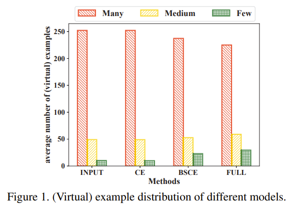
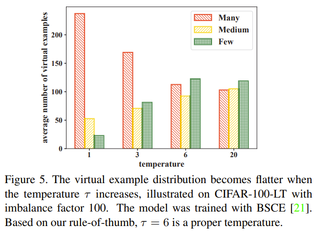
The authors propose the Distill the Virtual Examples (DiVE) method, which tackles long-tailed recognition by distilling knowledge from a teacher model's predictions, treated as virtual examples, to a student model. The key ideas of DiVE are as follows: Virtual example interpretation: The teacher model's prediction scores for each class are interpreted as virtual examples. For instance, a prediction of (0.7, 0.3) for a dog image is interpreted as 0.7 dog virtual examples and 0.3 cat virtual examples. This allows for direct interaction between classes, even if they are not semantically related. Equivalence between knowledge distillation and label distribution learning: The authors prove that under certain constraints, distilling from virtual examples is equivalent to label distribution learning (LDL). LDL is a technique that learns from uncertain labels represented as a distribution over classes. Necessity of a balanced virtual example distribution: For long-tailed recognition, the virtual example distribution must be flatter than the original input distribution to remove bias against tail classes. The authors demonstrate this requirement through theoretical analysis and empirical experiments. Explicit control of virtual example distribution: DiVE directly tunes the virtual example distribution towards a flatter one using two techniques: a) Adjusting the temperature parameter in the softmax function, which controls the smoothness of the output distribution. b) Applying power normalization to the teacher's soft labels, which further balances the virtual example distribution. Rule-of-thumb for determining flatness: The authors provide a rule-of-thumb for selecting the appropriate temperature and power normalization settings. The goal is to make the average number of virtual examples per category in the tail part slightly higher than that in the head part. Two-stage training pipeline: DiVE first trains a teacher model using any existing long-tailed recognition method (e.g., balanced softmax cross-entropy loss). Then, it distills the knowledge from the teacher's virtual examples to a student model using the DiVE loss function, which combines the balanced softmax cross-entropy loss and the KL divergence between the teacher and student predictions. The proposed DiVE method is simple yet effective, consistently outperforming state-of-the-art methods on various long-tailed benchmark datasets. The virtual example interpretation allows for explicit interaction between head and tail classes, while the control over the virtual example distribution ensures a more balanced learning process.

Problem Deep neural networks often perform poorly on long-tailed recognition tasks, where the number of samples per class varies significantly. Existing methods that address this issue by re-sampling or re-weighting training examples do not allow for direct interaction between head and tail classes, limiting their effectiveness.

Images

CUDA: Curriculum of Data Augmentation for Long-tailed Recognition

BibTex
@inproceedings{ahn2022cuda,
title={CUDA: Curriculum of Data Augmentation for Long-tailed Recognition},
author={Ahn, Sumyeong and Ko, Jongwoo and Yun, Se-Young},
booktitle={The Eleventh International Conference on Learning Representations},
year={2022}}

url=https://openreview.net/pdf?id=RgUPdudkWlN
Summary

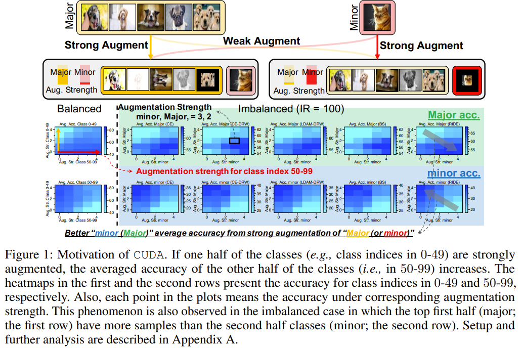
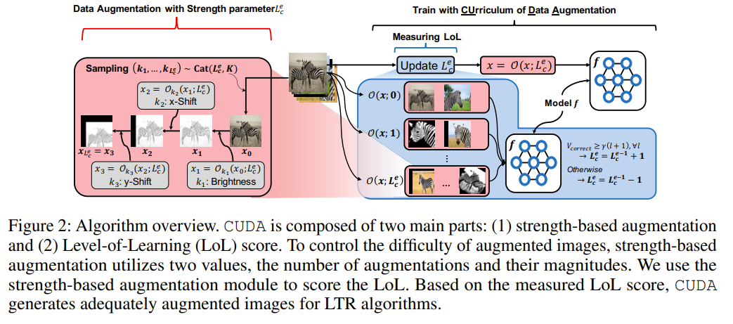
The authors propose CUDA (CUrriculum of Data Augmentation), a simple and efficient method for finding the appropriate per-class strength of data augmentation in long-tailed recognition tasks. The key ideas of CUDA are as follows: Strength-based data augmentation: CUDA controls the difficulty of augmented images using two values: the number of augmentations and their magnitudes. This allows for generating augmented samples with varying levels of difficulty. Level-of-Learning (LoL) score: CUDA introduces the LoL score, which measures how well the model can correctly predict augmented versions of samples from each class without losing the original information. The LoL score is adaptively updated during training. Curriculum learning: Based on the LoL score, CUDA increases the augmentation strength for classes that the model successfully predicts and decreases the strength for classes with incorrect predictions. This curriculum learning approach helps the model learn from easier samples first and gradually progress to more difficult augmented samples. Class-wise augmentation: CUDA applies augmentation strengths to each class independently, allowing the model to allocate appropriate levels of augmentation for different classes based on their learning progress. Compatibility with existing methods: CUDA can be easily integrated with various long-tailed recognition methods, such as class-balanced loss, two-stage training, and ensemble approaches, to further improve their performance. CUDA is trained in an end-to-end manner, where the LoL score is computed for each class at every epoch, and the augmentation strengths are determined accordingly. The proposed method is evaluated on several long-tailed benchmarks, demonstrating improved generalization performance compared to state-of-the-art methods.

Problem Conventional deep learning algorithms often suffer from performance degradation when trained on imbalanced datasets, where the number of samples per class varies significantly. Existing methods that aim to balance the impact of different classes by re-weighting or re-sampling training samples may not effectively capture the limited information in minority classes. Although some methods have attempted to augment minority classes by transferring information from majority classes, there has been limited analysis on determining which classes should be augmented and to what extent.

Images

TabNet: Attentive Interpretable Tabular Learning

BibTex
@inproceedings{arik2021tabnet,
title={Tabnet: Attentive interpretable tabular learning},
author={Arik, Sercan {\"O} and Pfister, Tomas},
booktitle={Proceedings of the AAAI conference on artificial intelligence},
year={2021}}

url=https://ojs.aaai.org/index.php/AAAI/article/download/16826/16633
Summary

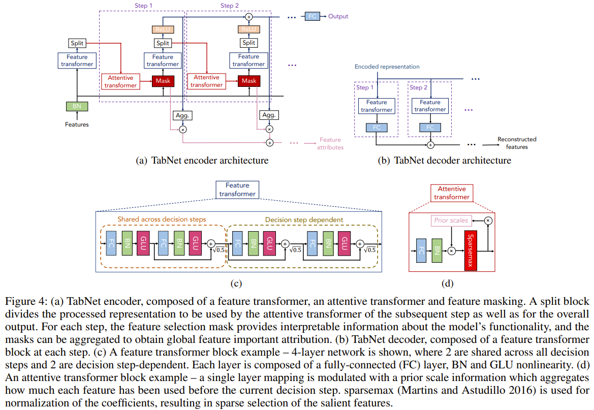
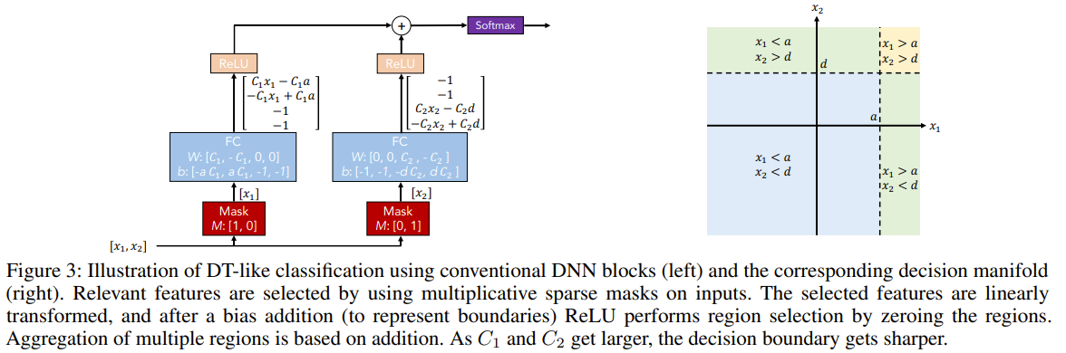
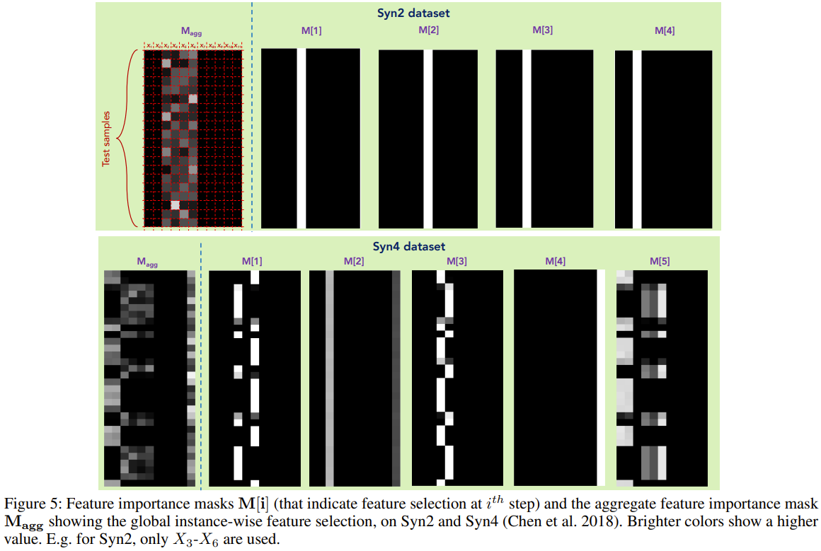
The authors propose TabNet, a novel deep learning architecture for tabular data that uses sequential attention to select salient features at each decision step, enabling interpretability and efficient learning. The key components of TabNet are: 1. Feature selection: TabNet employs a learnable mask to perform soft selection of salient features at each decision step. The mask is obtained using an attentive transformer that takes the processed features from the previous step as input. The masks are sparse, which allows the model to focus on the most relevant features and improves parameter efficiency. 2. Feature processing: The selected features are processed using a feature transformer, which consists of decision step-dependent and shared layers. The processed features are then split into the decision step output and information for the subsequent step. 3. Interpretability: TabNet's feature selection masks provide insight into the model's reasoning process. The masks can be analyzed at each decision step to understand the importance of individual features, and the masks can be aggregated to obtain global feature importance. 4. Tabular self-supervised learning: TabNet introduces a decoder architecture for reconstructing tabular features from the encoded representations. The model is trained to predict missing feature columns from the others, enabling unsupervised pre-training to improve performance when labeled data is scarce. The overall TabNet architecture consists of an encoder with multiple decision steps, each performing feature selection and processing, followed by an aggregation of the decision step outputs to obtain the final prediction. The model is trained end-to-end using standard classification or regression loss functions, along with a sparsity regularization term to encourage sparsity in the feature selection masks.

Problem Despite the remarkable success of deep neural networks (DNNs) in various domains, their performance on tabular data has been limited compared to tree-based ensemble methods. Tabular data often has complex relationships between features and target variables, with decision boundaries well-approximated by axis-aligned splits. Standard DNN architectures struggle to learn optimal decision boundaries for tabular data and lack interpretability, hindering their adoption in real-world applications.

Images

Local contrastive feature learning for tabular data

BibTex
@inproceedings{gharibshah2022local,
title={Local contrastive feature learning for tabular data},
author={Gharibshah, Zhabiz and Zhu, Xingquan},
booktitle={Proceedings of the 31st ACM International Conference on Information \& Knowledge Management},
year={2022}}

url= https://dl.acm.org/doi/pdf/10.1145/3511808.3557630?casa_token=1Z0XoSMMHn0AAAAA:5Vt7BZgpIoonKWOI5ML4Bjg8quihpVoVKJlCwNLSaxJkPUupQNLrQE-2fLb5V4t0Xxtivj5bOa7stA
Summary

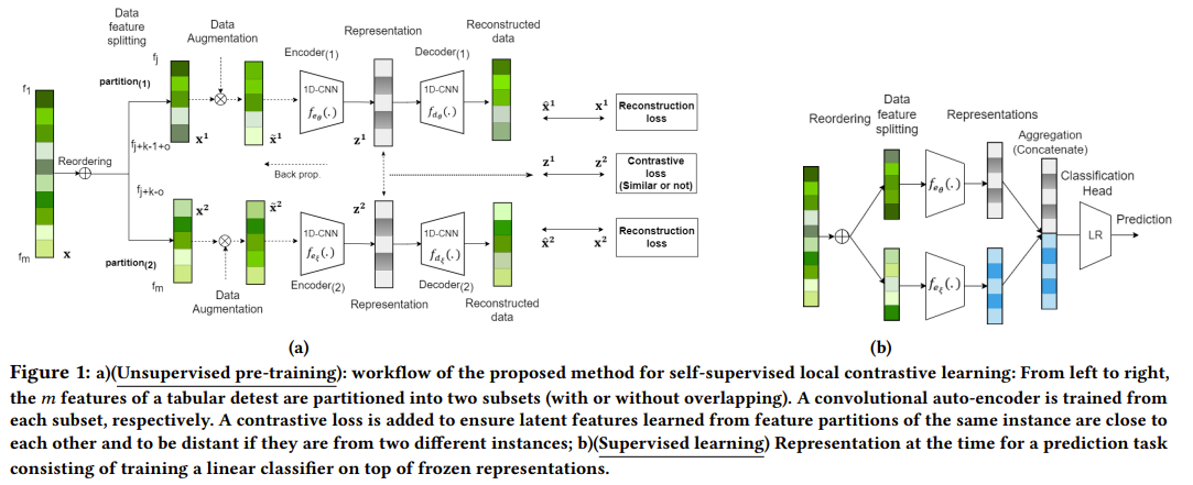
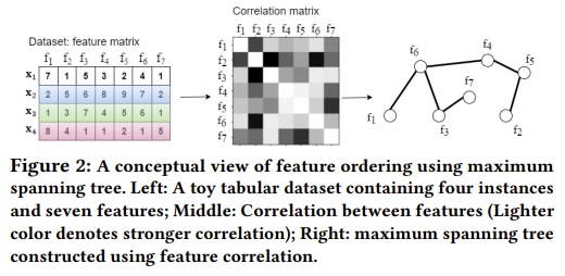
Gharibshah and Zhu propose a novel self-supervised representation learning framework called Local Contrastive Learning (LoCL) for tabular data. The key idea behind LoCL is to learn local patterns and features from subsets of features, exploiting the inherent correlations and interactions often present in real-world tabular datasets. The LoCL framework consists of several key components. First, to enable local learning, the input features are reordered based on their pairwise Pearson correlation coefficients. This is achieved by constructing a maximum spanning tree, where features are treated as nodes and the absolute values of correlations as edge weights. The tree is then traversed using a depth-first search starting from the feature pair with the highest correlation, yielding a new feature order that places strongly correlated features adjacent to each other. Next, the reordered features are partitioned into subsets, allowing local patterns to be learned from groups of correlated features. The authors suggest using two subsets, although the framework can accommodate more. Each feature subset is then processed by a separate 1D convolutional autoencoder branch. The autoencoders learn latent representations that capture the local structure within each subset. To train the autoencoders, LoCL employs a combination of two loss functions in a self-supervised manner. The first is a contrastive loss, which maximizes the agreement between the latent representations of different feature subsets from the same instance. Specifically, the contrastive loss encourages the latent representations of the two feature subsets to be similar for the same instance and dissimilar for different instances. The second loss term is a reconstruction loss that is applied separately to each feature subset. It ensures that the learned representations can accurately reconstruct the original input features within each subset. The total loss is a weighted sum of the contrastive and reconstruction losses. Finally, to obtain the overall representation for a given instance, the latent representations from each autoencoder branch are concatenated. This final representation, which captures both local patterns within feature subsets and global interactions between subsets, can then be used for various downstream tasks such as classification or anomaly detection.

Problem Existing self-supervised representation learning methods for tabular data typically use dense neural networks to learn global patterns from all features. However, in many real-world datasets, useful patterns often only involve a small subset of features, and features frequently exhibit local correlations and interactions. Dense networks struggle to effectively capture these local patterns. There is a need for a self-supervised learning approach that can leverage the local structure and correlations in tabular features to learn more informative representations.

Images

Learning Enhanced Representations for Tabular Data via Neighborhood Propagation

BibTex
@article{du2022pet,
title={Learning enhanced representation for tabular data via neighborhood propagation},
author={Du, Kounianhua and Zhang, Weinan and Zhou, Ruiwen and Wang, Yangkun and Zhao, Xilong and Jin, Jiarui and Gan, Quan and Zhang, Zheng and Wipf, David P},
journal={Advances in Neural Information Processing Systems},
year={2022}}

url= https://proceedings.neurips.cc/paper_files/paper/2022/file/67e79c8e9b11f068a7cafd79505175c0-Paper-Conference.pdf
Summary

The paper proposes PET (Propagate and Enhance Tabular data), a novel architecture that constructs a retrieval-based hypergraph to model cross-row and cross-column relationships, and propagates information on the graph to enhance target data representations for prediction. PET is particularly effective when, at inference time, nearest neighbor data is available (e.g., a running memory of data), and the data instances are not assumed to be independent and identically distributed (non-IID). The key components of PET are:
1. Retrieval-based hypergraph construction: For each target data instance, PET retrieves a set of relevant instances based on a relevance metric. The relevance metric assigns higher weights to matches of rarer feature values because it is harder to match them compared to more frequent feature values, making their matches more meaningful. The resulting instance set is modeled as a hypergraph, where each distinct feature value forms a node and each data instance (a collection of feature values) forms a hyperedge. The hypergraph is then transformed into a bipartite graph through star expansion, where the two sets of vertices represent feature values and data instances, respectively.
2. Message passing and interaction: PET performs message propagation on the bipartite graph to enhance data representations. The propagation serves three purposes:
a) Label propagation: Labels from retrieved instances propagate through common feature value nodes to help predict the target instance's label.
b) Feature enhancement: Features are enhanced by capturing high-order interactions through the graph structure. The interactive message generation, attention-based aggregation, and node embedding update steps generate locality-aware high-order feature interactions.
c) Label-feature interaction: Labels are incorporated into the propagating messages to adjust feature spaces and generate label-enhanced feature representations.

3. Prediction: After message passing, the enhanced target data instance representation is used for the final prediction.
The proposed propagation mechanism in PET allows for effective utilization of label information and feature interactions across data instances. By modeling the relationships among instances and propagating information through the graph, PET learns more informative and discriminative representations for tabular data prediction. In essence, PET can be viewed as a Graph Neural Network (GNN) based feature extractor that leverages the relationships among data instances and their feature values to learn enhanced representations. PET to learn more expressive and informative representations for improved tabular data prediction, especially in non-IID settings where nearest neighbor data is available at inference time. However, the additional steps involved in retrieval and graph construction make the inference process slower compared to methods that treat data instances independently.

Problem Problem: Prediction over tabular data is a fundamental problem in many applications. However, most existing methods either treat each data instance independently without considering the relationships among them, or do not effectively utilize the information from multiple instances to enhance the target representation for prediction. This limits their ability to capture cross-row and cross-column patterns in tabular data.

Images

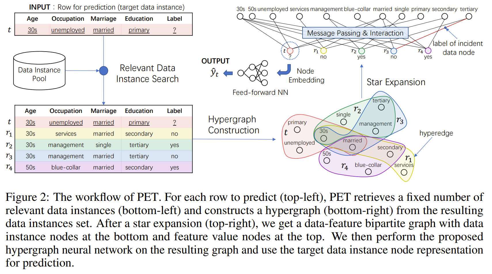
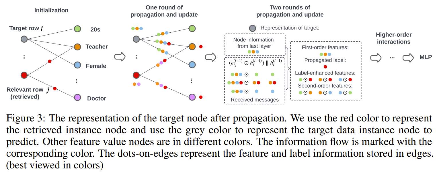
Multidimensional Scaling by Optimizing Goodness of Fit to a Nonmetric Hypothesis

BibTex
@article{kruskal1964mds,
title={Multidimensional scaling by optimizing goodness of fit to a nonmetric hypothesis},
author={Kruskal, Joseph B},
journal={Psychometrika},
publisher={Springer}
year={1964}}

url1=http://cda.psych.uiuc.edu/psychometrika_highly_cited_articles/kruskal_1964a.pdf
url2=http://cda.psych.uiuc.edu/psychometrika_highly_cited_articles/kruskal_1964b.pdf
Summary

MDS paper 1 Objective one is finding d_hat given config such that monotonicity with the object dissimilarity is maintained (<=, not just <) Objective two is finding a configuration X (x_il in NT-dimensional space) to minimize the stress Consequence 1: MDS doesn’t take into account the object’s features themselves but just their dissimilarity rankings Consequence 2: MDS through Algo 1 for objective 2 finds the feature values of the configuration (representations) directly, not the weights of a Model that generates the feature values of the representations. MDS paper 2 Objective 1 is achieved by forming blocks such that Block b is up-satisfied, or the d_hat value of b is less than the d_hat value of the block following b Block b is down-satisfied, or the d_hat value of b is higher than the ed_hat value of the block preceding b Starting with each point as a block, the blocks are merged with their neighboring blocks if they are either not up-satisfied or down-satisfied Objective 2 is achieved by gradient descent, the gradient of the stress with respect the the configuration feature values. The step side has 3 additional factors, which are, Angle factor, which considers the similarity between consecutive gradients Relaxation factor which considers the ratio between current stress and stress from 5 iterations ago. Good luck factor, which considers the ratio between current stress and the previous iteration stress.

Problem Find a dimensional representation of objects that maintains the rank order of their dissimilarities while minimizing a stress function.

Images

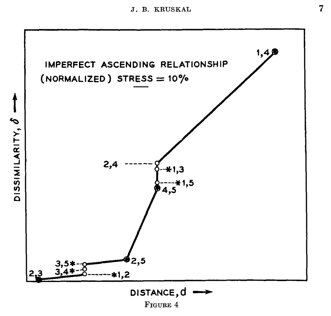
Visualizing data using t-SNE

BibTex
@article{van2008tsne,
title={Visualizing data using t-SNE.},
author={Van der Maaten, Laurens and Hinton, Geoffrey},
journal={Journal of machine learning research},
year={2008}}

url=https://www.jmlr.org/papers/volume9/vandermaaten08a/vandermaaten08a.pdf?fbcl
Summary

The paper introduces t-Distributed Stochastic Neighbor Embedding (t-SNE), a novel technique designed to improve the visualization of high-dimensional data by mapping it into a lower-dimensional space. t-SNE addresses significant challenges in existing methods, particularly the crowding problem and the difficulty of preserving both local and global structures. The crowding problem arises because, in high-dimensional spaces, the volume increases exponentially with the radius, leading to many points being equidistant from a central point. In low-dimensional visualizations, this results in points being placed too closely together. To begin, t-SNE converts high-dimensional data into a matrix of pairwise similarities, employing conditional probabilities based on Gaussian distributions. Each high-dimensional data point selects its neighbors with probabilities proportional to their similarity, modeled using a Gaussian distribution centered on the point. These probabilities are then symmetrized to ensure mutual comparability between any two points. In the low-dimensional space, t-SNE uses a Student-t distribution to represent similarities, effectively handling the crowding problem by spreading out the points more appropriately. This allows moderate distances in high-dimensional space to be faithfully represented by larger distances in the low-dimensional map, thus preserving both local and global structures. The optimization of the t-SNE cost function is performed using a gradient descent method with a momentum term. Two key techniques, early compression and early exaggeration, are employed to enhance the optimization process. Early compression involves applying an additional penalty to keep all points close to the origin at the start. This helps clusters explore the space more freely and settle into a more globally optimal configuration. The penalty is gradually reduced to allow points to spread out appropriately. Specifically, an L2-penalty is added to the cost function, proportional to the sum of squared distances of the map points from the origin, and is reduced over iterations. Early exaggeration, on the other hand, involves multiplying all pairwise similarities by a constant factor (e.g., 4) during the initial optimization phase. This exaggeration strengthens the attractive forces between similar points, encouraging the formation of tight, distinct clusters. Once the clusters are formed, the exaggeration is removed, allowing for fine-tuning of the map. To handle large datasets, the paper introduces a "landmark" approach, which uses random walks on neighborhood graphs to visualize subsets of the data while maintaining the overall structure. This approach selects a subset of data points (landmarks) and initiates random walks from these landmarks to compute similarities based on the entire dataset. By integrating information from all data points, not just the landmarks, this method ensures that the global structure influences the visualization. The probabilities of transitioning between landmarks are calculated by considering paths through all data points, making the visualization robust to the overall data structure. Despite its strengths, t-SNE has potential weaknesses, including sensitivity to the intrinsic dimensionality of data and the non-convexity of its cost function. Future work aims to optimize the degrees of freedom in the Student-t distribution, extend t-SNE to higher dimensions, and develop a parametric version for better generalization.

Problem The problem of visualizing high-dimensional data lies in effectively reducing the data to a lower-dimensional space while preserving its significant structure. Prior methods often struggle with retaining both the local and global structures of the data, leading to issues like the crowding problem and difficulty in separating clusters in the visualized map.

Images

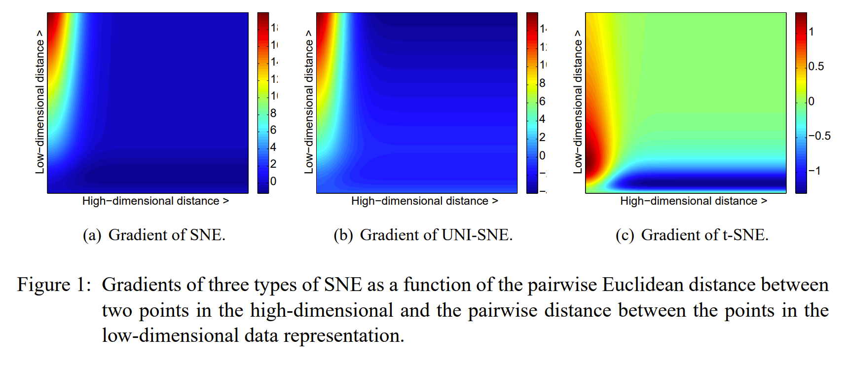
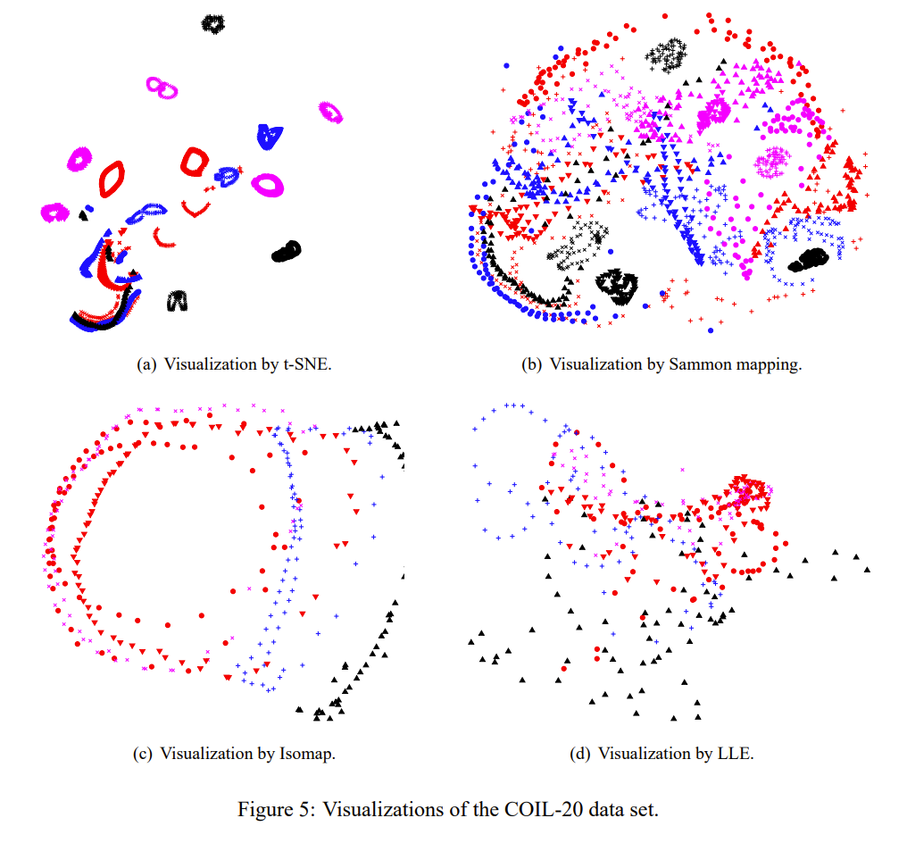
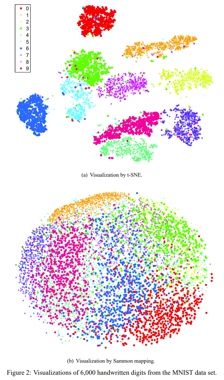
ConR: Contrastive Regularizer for Deep Imbalanced Regression

BibTex
@article{keramati2023conr,
title={Conr: Contrastive regularizer for deep imbalanced regression},
author={Keramati, Mahsa and Meng, Lili and Evans, R David},
booktitle={International Conference on Learning Representations},
year={2024}}

url=https://openreview.net/pdf?id=RIuevDSK5V
Summary

The paper introduces ConR, a novel contrastive regularizer designed to address deep imbalanced regression (DIR) by effectively modeling both local and global label similarities in the feature space. ConR aims to prevent minority sample features from collapsing into majority sample features, a common issue in imbalanced regression tasks. It operates by penalizing incorrect proximities in the feature space proportionally to label similarities while encouraging correct proximities to model local similarities. ConR builds upon the concept of contrastive learning, utilizing problem-specific augmentations to create pairs of augmented samples. For each augmented sample, ConR performs two levels of subset selection: Negative Pair Selection: Negative pairs are selected based on prediction similarities. A pair is considered negative if the examples have dissimilar labels but similar predictions. Anchor Selection: An anchor is chosen if it has at least one negative pair. Specifically, anchors are selected from samples exhibiting confusion around their feature space position, meaning they have misclassified predictions. The regularizer applies a loss function that pulls together positive pairs (samples with similar labels) and pushes away negative pairs (samples with dissimilar labels but similar predictions). The pushing force is determined by a similarity threshold, which defines whether pairs are considered similar or dissimilar. ConR is implemented as a regularizer, meaning it is added to the primary regression loss function to enhance the model's learning process. The pushing weight for negative pairs does not solely depend on label dissimilarity but also on the anchor's label density. This weight is computed as the product of a density-based weight for the anchor and the inverse of the label similarity between the anchor and the negative pair. This approach ensures that minority samples, which typically have lower density, exert a stronger repulsion force on their negative pairs, helping to maintain a balanced feature space. Additionally, the inverse label similarity factor ensures that samples with highly dissimilar labels from the anchor exert a stronger repulsion, thus maintaining the integrity of the feature space across diverse label distributions. A key finding from the ablation studies is that the biggest contributor to ConR's effectiveness is the selection of negative examples to focus solely on mistakes. By concentrating on these errors, ConR significantly enhances the learning process, leading to better model performance.

Problem Existing methods for imbalanced data primarily address categorical labels and struggle to generalize to deep imbalanced regression (DIR) tasks, where the label space is continuous, leading to the collapse of minority samples into their majority counterparts.

Images

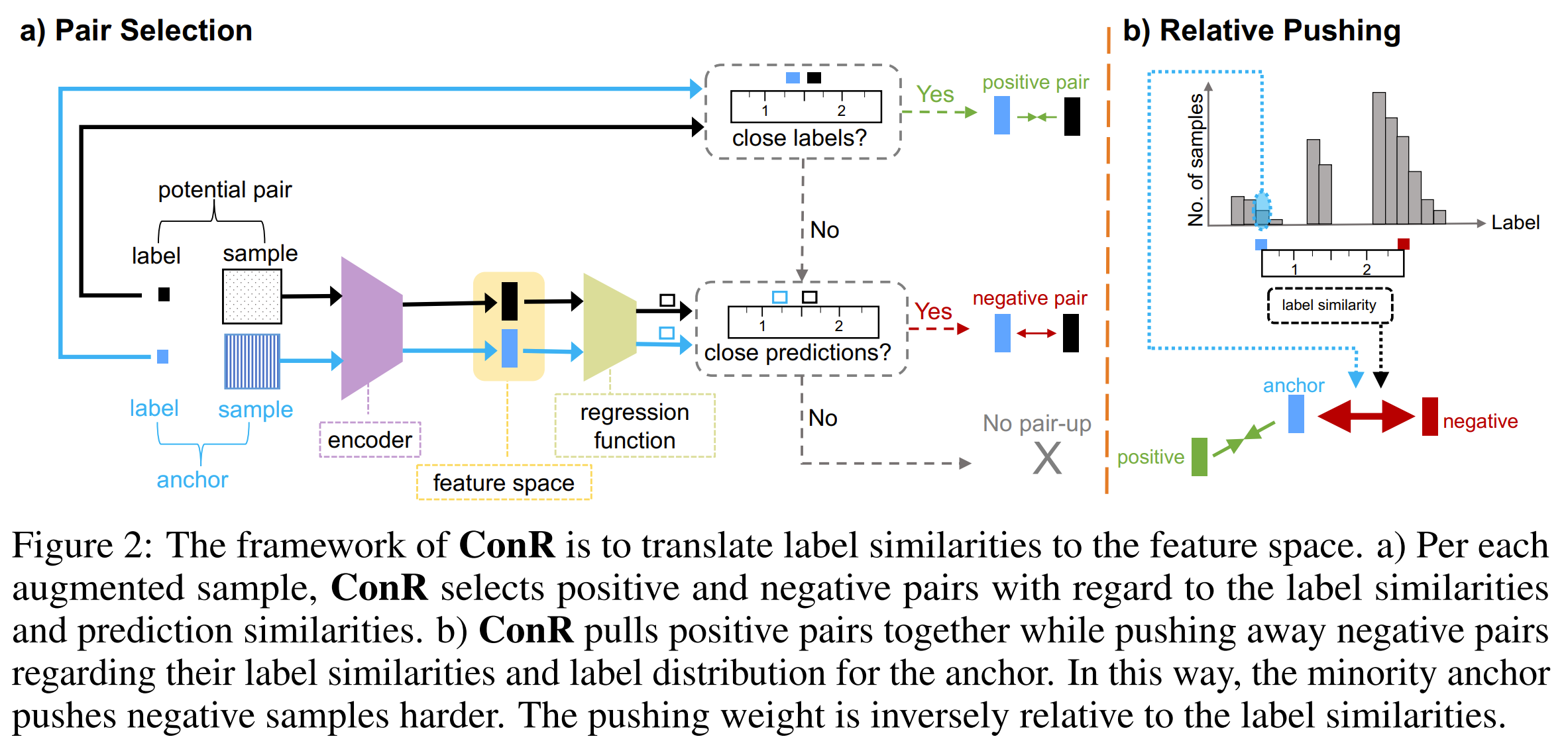
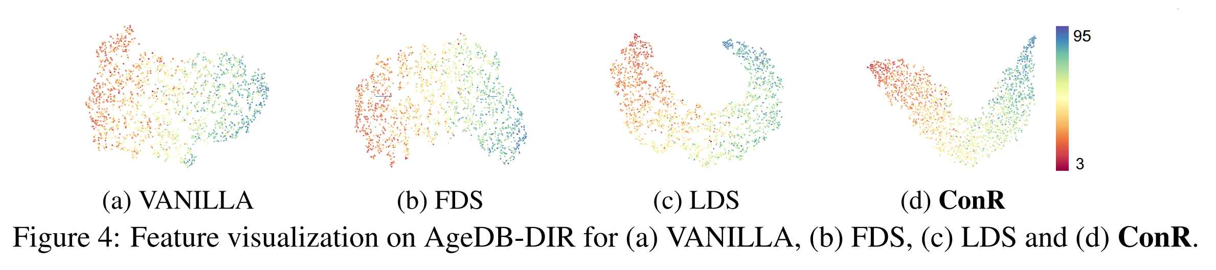
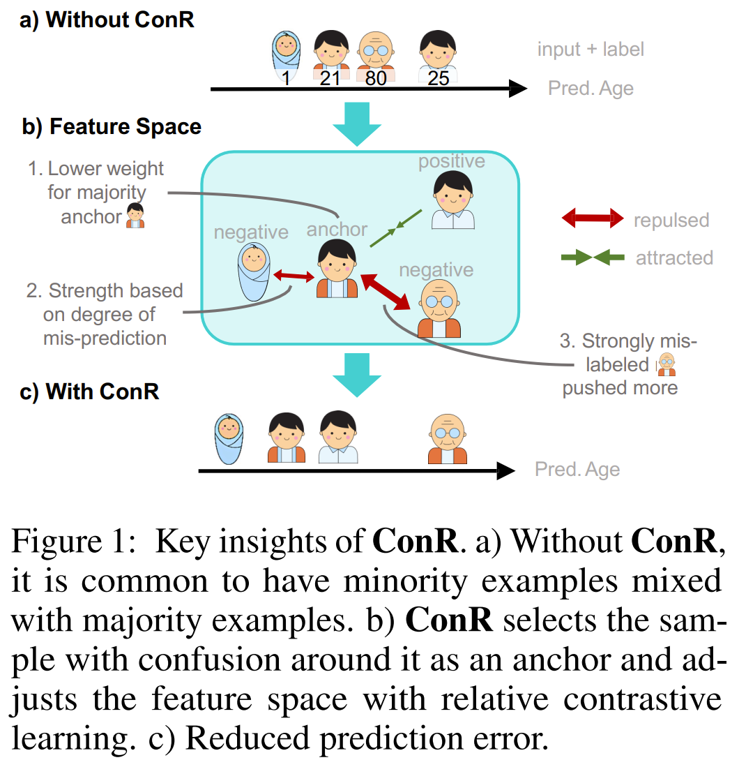
Simplifying Neural Network Training Under Class Imbalance

BibTex
@article{shwartz2023sama,
title={Simplifying Neural Network Training Under Class Imbalance},
author={Shwartz-Ziv, Ravid and Goldblum, Micah and Li, Yucen and Bruss, C Bayan and Wilson, Andrew G},
journal={Advances in Neural Information Processing Systems},
year={2023}}

url=https://openreview.net/pdf?id=iGmDQn4CRj
Summary

The paper investigates the persistent challenge of class-imbalanced datasets in neural network training, where certain classes are significantly underrepresented, leading to suboptimal model performance. Traditional approaches to this issue have largely focused on developing specialized loss functions and sampling techniques. In contrast, this paper proposes a novel methodology that involves fine-tuning existing components of standard training routines to achieve superior performance without the need for such specialized methods. The authors highlight several key adjustments to standard training routines. First, they demonstrate that smaller batch sizes can effectively mitigate overfitting to majority classes in imbalanced settings by acting as a regularizer. Despite smaller batches not always containing minority class samples, their regularizing effect is particularly beneficial. Data augmentation is another critical component examined in the study. The authors find that augmentation techniques, especially those like AutoAugment, significantly enhance performance on imbalanced datasets by improving minority class accuracy. This finding underscores the importance of selecting appropriate augmentation policies tailored to the level of class imbalance. A noteworthy contribution of the paper is the integration of self-supervised learning (SSL) during training. By combining supervised learning with an additional SSL loss function, the authors improve feature representations and generalization, particularly for minority classes. This joint SSL approach eliminates the need for extensive pre-training on large, balanced datasets and directly enhances performance in class-imbalanced contexts. Sharpness-Aware Minimization (SAM) is adapted to address class imbalance more effectively. The adapted method, termed SAM-Asymmetric (SAM-A), focuses more on minority class loss terms, creating wider decision boundaries around minority samples and preventing overfitting. This adjustment is shown to be highly effective in improving minority class performance. Additionally, the paper proposes the use of label smoothing, particularly aggressive smoothing for minority class examples. This technique reduces the confidence of the model on minority class predictions, promoting better generalization and preventing overfitting.
The findings of the study reveal several important insights. Smaller batch sizes are particularly effective in imbalanced settings, and data augmentation significantly boosts minority class accuracy. Larger model architectures, while beneficial for balanced datasets, tend to overfit on imbalanced data. Self-supervised pre-training methods offer substantial benefits, with SSL pre-training yielding better generalization than supervised pre-training. The adapted SAM and label smoothing strategies further enhance performance by promoting wider decision boundaries and reducing overfitting.

Problem This paper addresses the challenge of improving neural network performance on class-imbalanced datasets by demonstrating that fine-tuning standard training components—such as batch size, data augmentation, optimizer settings, and label smoothing—can achieve state-of-the-art results without the need for specialized loss functions or sampling techniques.

Images

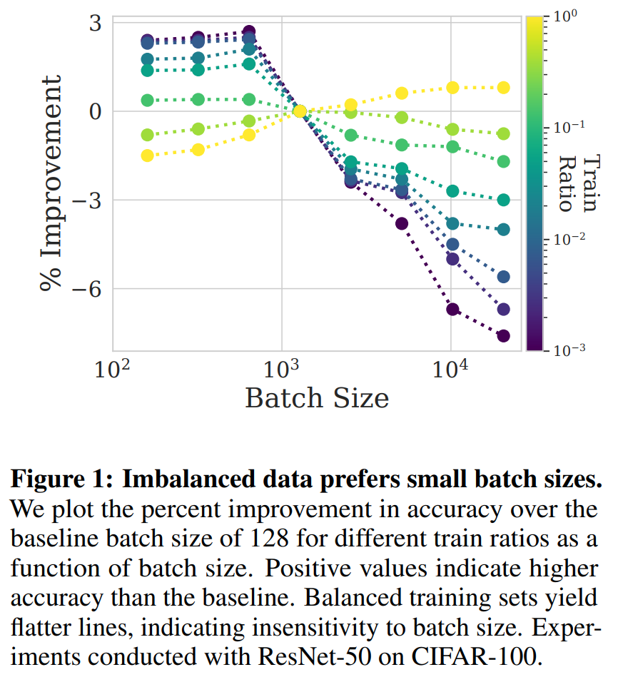
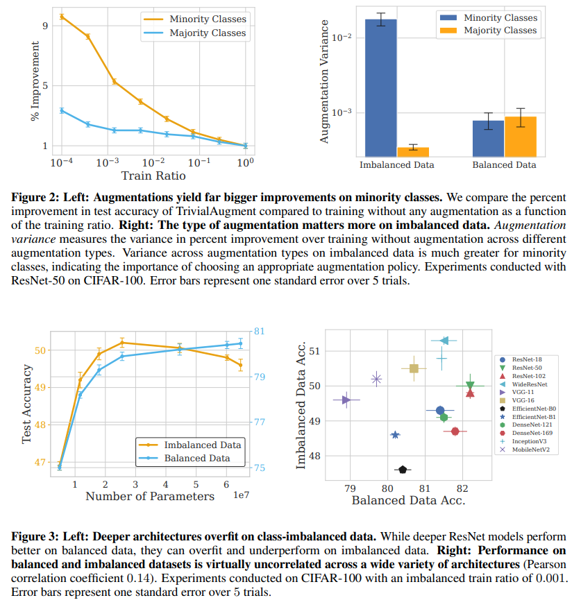
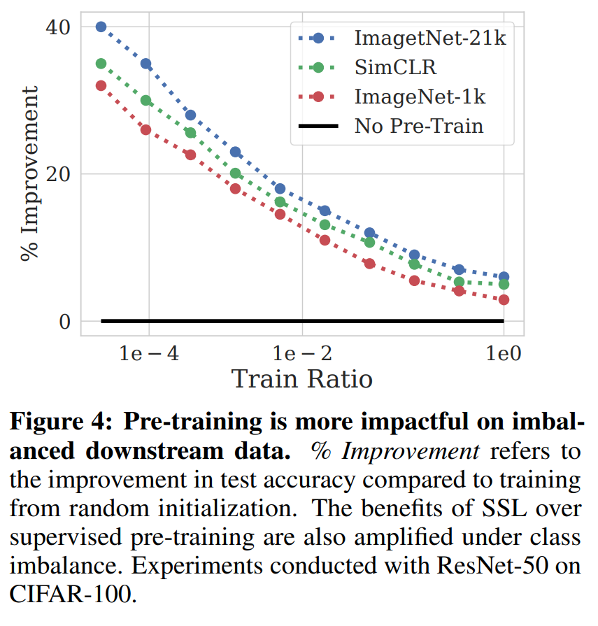
How Re-sampling Helps for Long-Tail Learning?

BibTex
@article{shi2023csa,
title={How Re-sampling Helps for Long-Tail Learning?},
author={Shi, Jiang-Xin and Wei, Tong and Xiang, Yuke and Li, Yu-Feng},
journal={Advances in Neural Information Processing Systems},
year={2023}}

url= https://proceedings.neurips.cc/paper_files/paper/2023/file/eeffa70bcbbd43f6bd067edebc6595e8-Paper-Conference.pdf
Summary

The authors conducted a series of experiments on various datasets, including MNIST-LT, Fashion-LT, CIFAR100-LT, and ImageNet-LT, to analyze the effects of re-sampling. They observed that when training samples included irrelevant contexts, such as backgrounds not related to the main subject, re-sampling tended to overfit these contexts, leading to poor performance. Conversely, when training images were highly correlated with their target labels, class-balanced re-sampling helped in learning more discriminative feature representations. This dual behavior highlighted the need for a nuanced approach to re-sampling. To address the issue of spurious correlations learned from irrelevant contexts, the authors proposed a novel context-shift augmentation module. This module operates in two main phases. In the first phase, a uniform sampling model is used to extract the background (irrelevant context) from head-class images. This extraction process employs techniques like Grad-CAM, which finds features important to the prediction and subtracts them out to obtain the background. The resulting irrelevant contexts are then stored in a context bank. In the second phase, the extracted irrelevant contexts are combined with tail-class images during re-sampling to generate new, diverse training samples. The combination is kept random with a lambda parameter and the background is kept continuous (ranging from 0 to 1) for a more fuzzy combination. Mixup is added to accurately depict the label of this fuzzy combination. This process ensures that the model does not overfit the irrelevant contexts and instead learns to distinguish the tail classes better. The proposed context-shift augmentation module was validated through extensive experiments on long-tail versions of CIFAR10, CIFAR100, and ImageNet datasets. The results demonstrated that the module outperforms traditional class-balanced re-sampling and other methods, including Classifier Re-Training (cRT) and various data augmentation techniques like Mixup and Remix. These findings underscore the module's ability to improve the generalization ability of models trained on long-tail datasets. Interestingly, the authors found that irrelevant context is only an issue when the context is not shared between head and tail classes. When the context is actually shared between head and tail classes, there is no problem, as demonstrated in their experiments with the MNIST-LT dataset. This insight further refines the understanding of when and how re-sampling strategies can be effectively applied to long-tail learning scenarios.

Problem Re-sampling in long-tailed learning can lead to overfitting irrelevant context and thus reduce performance on the tail classes, necessitating methods to mitigate this problem.

Images

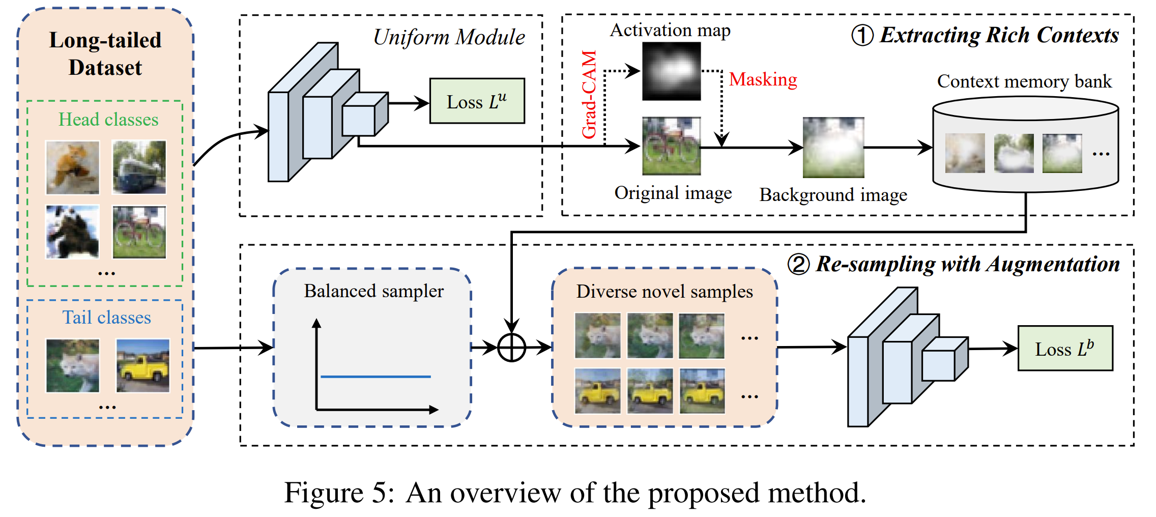
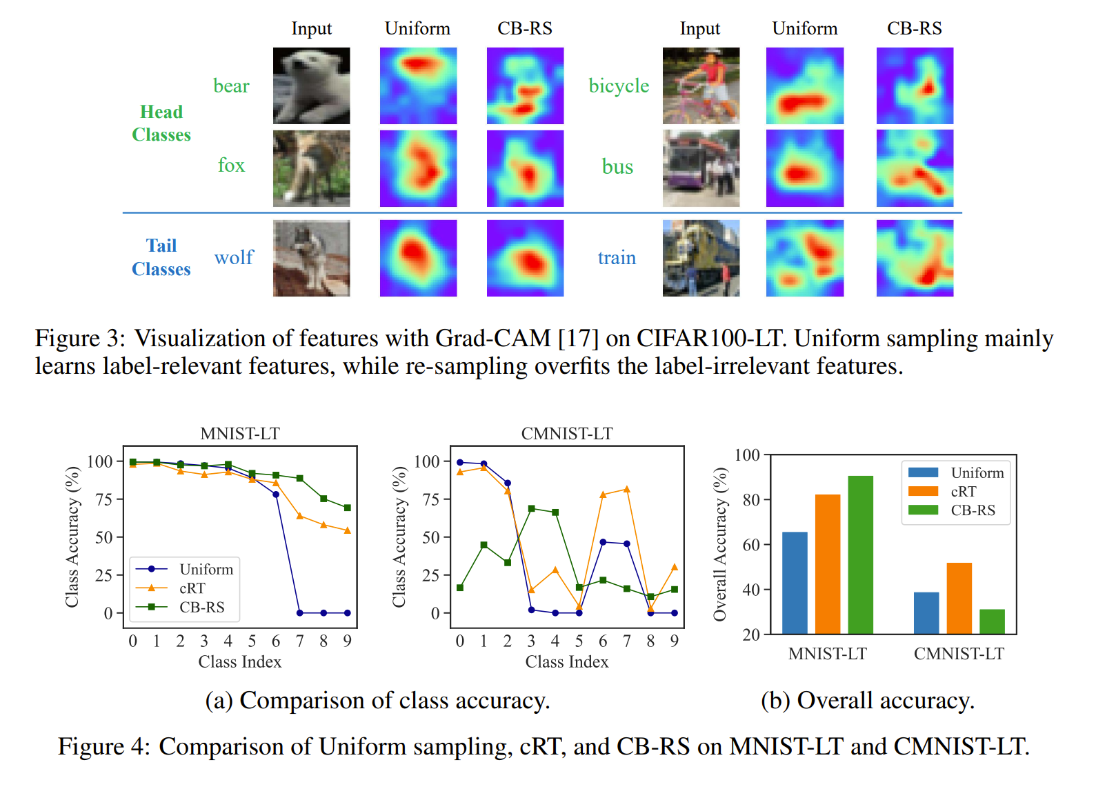
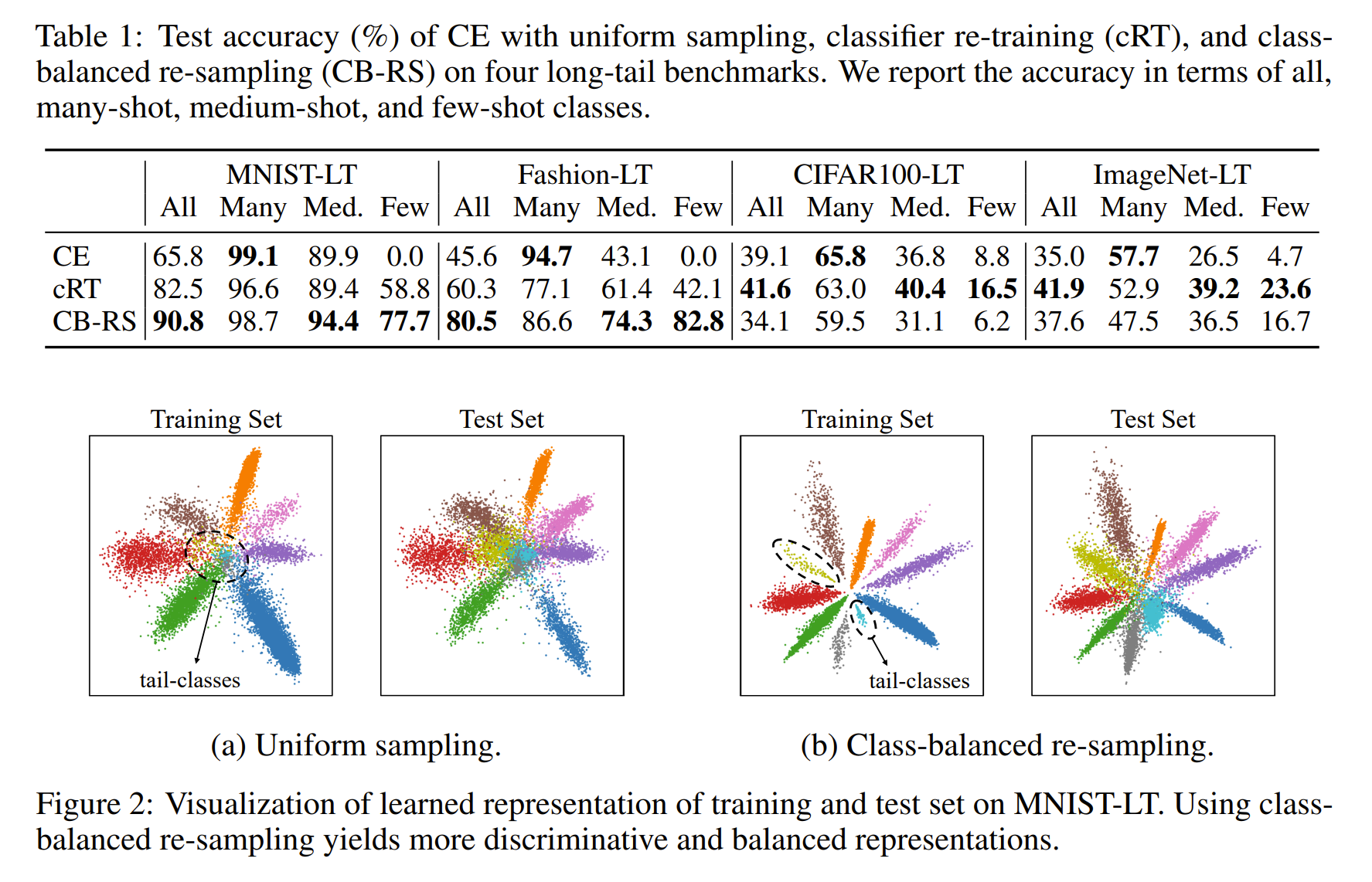
SimPer: Simple Self-Supervised Learning of Periodic Targets

BibTex
@inproceedings{yang2022simper,
title={SimPer: Simple Self-Supervised Learning of Periodic Targets},
author={Yang, Yuzhe and Liu, Xin and Wu, Jiang and Borac, Silviu and Katabi, Dina and Poh, Ming-Zher and McDuff, Daniel},
booktitle={The Eleventh International Conference on Learning Representations},
year={2023}}

url=https://openreview.net/pdf?id=EKpMeEV0hOo
Summary

SimPer, short for Simple Self-Supervised Learning of Periodic Targets, addresses the limitations of existing self-supervised learning (SSL) methods in capturing periodic or quasi-periodic information in data. Traditional SSL methods excel at discrete classification and segmentation tasks but fail to recognize and learn from the inherent periodicity in various datasets, such as those found in human physiology, environmental sensing, and human behavior analysis. SimPer fills this gap by introducing a new SSL regime tailored specifically for learning periodic representations. One of the key innovations in SimPer is the introduction of periodic feature similarity measures. Unlike conventional feature similarity measures like cosine similarity, which emphasize strict alignment of feature vectors, SimPer's periodic feature similarity accounts for the cyclical nature of periodic data. This means it retains high similarity scores for features even when their indexes are shifted or reversed, as long as the periodic information remains consistent. Two practical instantiations are Maximum Cross-Correlation (MXCorr), which measures the maximum similarity as a function of offsets between signals, and Normalized Power Spectrum Density (nPSD), which calculates the distance between the normalized power spectral densities of two feature vectors. These measures ensure that the learned representations accurately reflect the periodic characteristics of the data. SimPer also introduces periodicity-invariant and periodicity-variant transformations to construct positive and negative pairs for contrastive learning. Periodicity-invariant transformations preserve the underlying periodic signals while applying spatial or temporal changes, such as cropping, resizing, reversing, or delaying the sequence. These transformations generate positive pairs by creating different views of the same instance that maintain the same periodic information. On the other hand, periodicity-variant transformations alter the frequency of the input sequence, effectively changing the identity of the periodic targets. By modifying the speed of the sequence, these transformations produce negative pairs from the same instance, as the altered frequency results in different periodic signals. This approach enables SimPer to create a rich set of positive and negative examples, enhancing its ability to learn robust periodic representations. Additionally, SimPer employs a generalized contrastive loss function to better capture the continuous nature of frequency labels. Traditional contrastive loss functions like InfoNCE treat each sample pair as either positive or negative without considering the relative similarity between different negatives. In contrast, SimPer's generalized loss assigns a soft label to each pair based on their frequency distance, allowing for a more nuanced representation learning. This loss function contrasts over continuous targets by scaling the contributions of all pairs according to their label similarities, rather than treating each pair with a hard binary distinction. This approach helps SimPer learn more precise and meaningful periodic representations.

Problem how to effectively learn representations for periodic or quasi-periodic targets in data using self-supervised learning methods, which existing SSL methods fail to capture due to their oversight of intrinsic periodicity in data.

Images

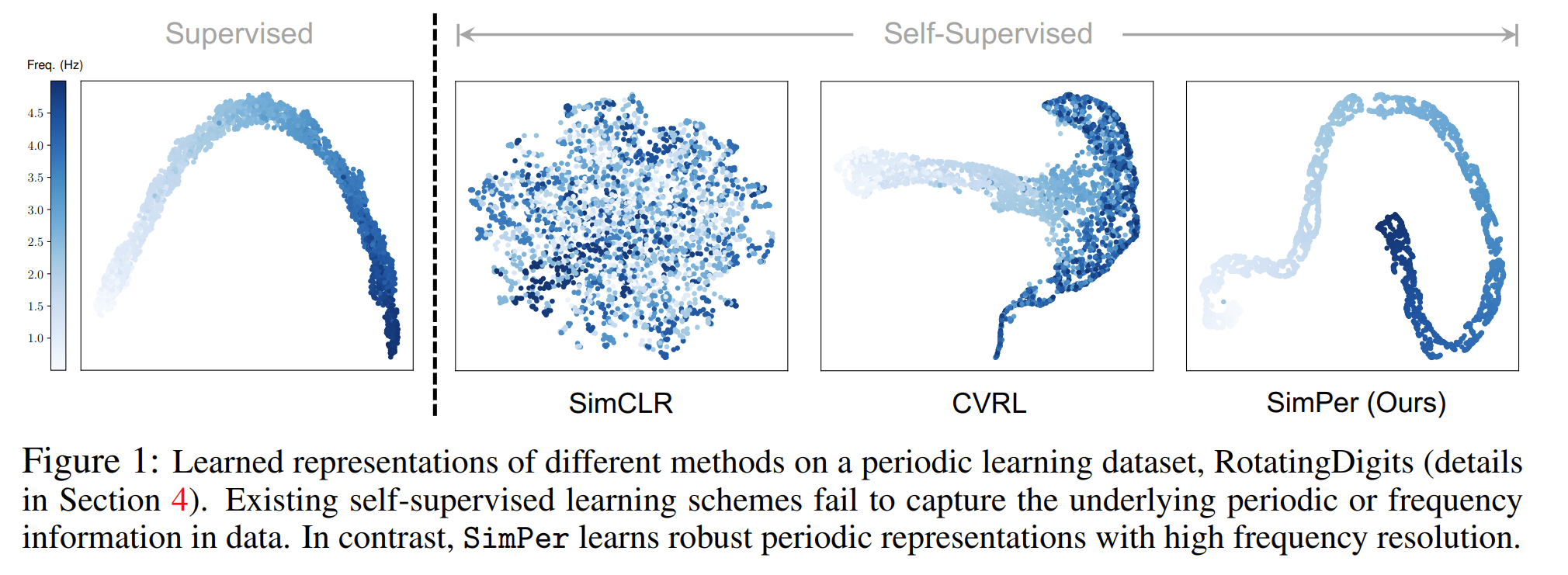
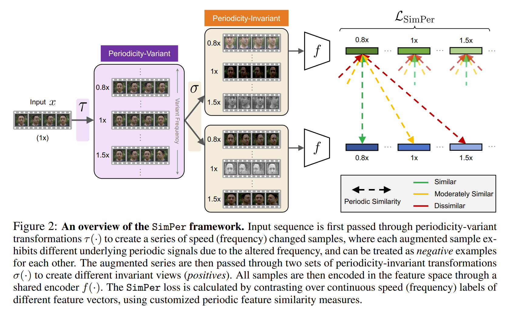
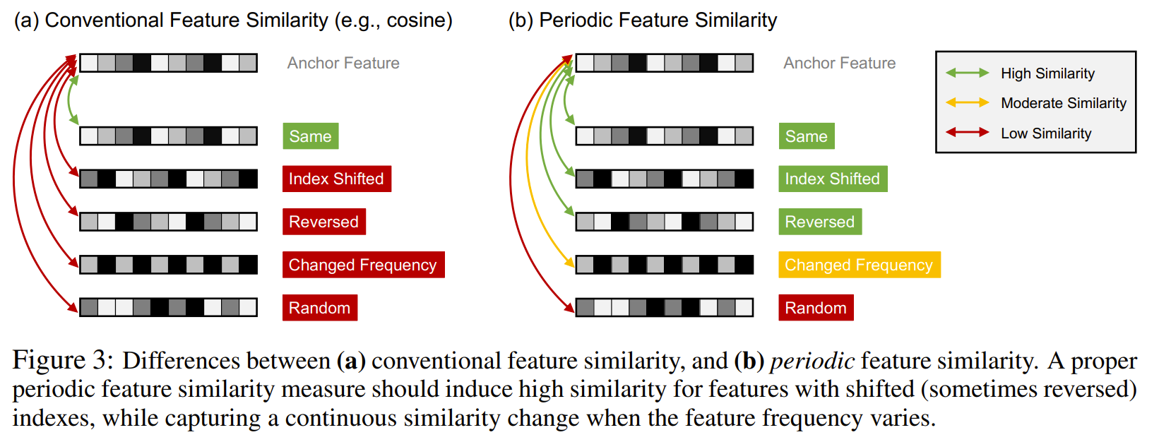
Sharpness-Aware Minimization for Efficiently Improving Generalization

BibTex
@inproceedings{foret2020SAM,
title={Sharpness-aware Minimization for Efficiently Improving Generalization},
author={Foret, Pierre and Kleiner, Ariel and Mobahi, Hossein and Neyshabur, Behnam},
booktitle={International Conference on Learning Representations}
year={2020}}

url=https://openreview.net/pdf?id=6Tm1mposlrM
Summary

Traditional optimization methods that focus solely on minimizing the training loss often result in sharp minima in the loss landscape, and these sharp minima are associated with poor generalization. The goal of SAM is to find flatter minima, which are correlated with better generalization performance. To address this issue, SAM simultaneously minimizes the value of the training loss and the sharpness of the loss landscape. The SAM method involves formulating a new objective that incorporates a term accounting for the sharpness of the loss. Specifically, the SAM objective is defined as the minimization of the maximum loss within a neighborhood of the current parameters.This formulation ensures that the parameters found by the optimization process not only minimize the loss but also reside in a neighborhood where the loss remains uniformly low, leading to flatter minima. To solve this SAM objective efficiently, the method approximates the gradient of the SAM objective by differentiating through the inner maximization problem. This involves computing the adversarial perturbation that maximizes the loss in the local neighborhood and then updating the model parameters in the direction that minimizes this perturbed loss. In the context of estimating sharpness, a larger the batch size used in the approximation provides a better estimate of the sharpness of the landscape, as it allows for a more comprehensive assessment of the local loss variations. The implementation of SAM involves two main steps for each parameter update. First, it computes the adversarial perturbation by performing a gradient ascent step on the loss. Second, it updates the model parameters using the gradient of the perturbed loss. These steps ensure that the optimization process is guided towards flatter regions of the loss landscape, improving generalization.

Problem Often models generalize poorly due to the sharp local minimum the converge to. Paper aims at improving the generalization ability of heavily overparameterized models by simultaneously minimizing loss value and loss sharpness to avoid suboptimal model quality.

Images

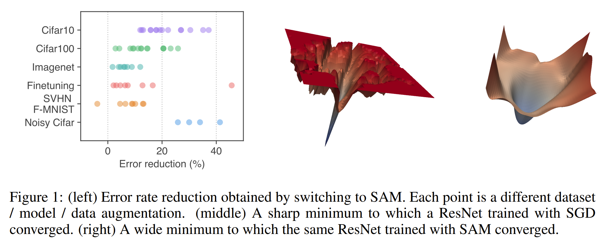
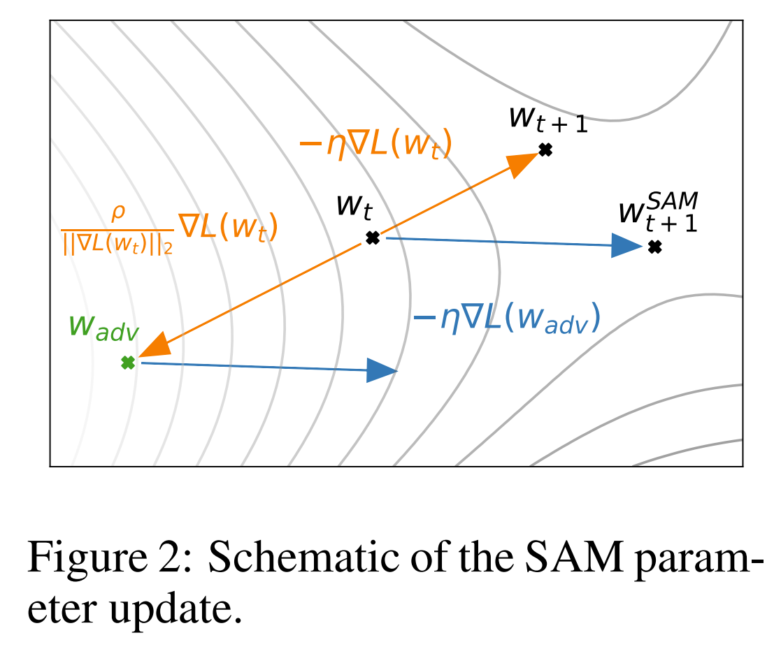
Class-Conditional Sharpness-Aware Minimization for Deep Long-Tailed Recognition

BibTex
@inproceedings{zhou2023ccsam,
title={Class-conditional sharpness-aware minimization for deep long-tailed recognition},
author={Zhou, Zhipeng and Li, Lanqing and Zhao, Peilin and Heng, Pheng-Ann and Gong, Wei},
booktitle={Proceedings of the IEEE/CVF Conference on Computer Vision and Pattern Recognition},
year={2023}}

url= https://openaccess.thecvf.com/content/CVPR2023/papers/Zhou_Class-Conditional_Sharpness-Aware_Minimization_for_Deep_Long-Tailed_Recognition_CVPR_2023_paper.pdf
Summary

The paper "Class-Conditional Sharpness-Aware Minimization for Deep Long-Tailed Recognition" introduces a novel two-stage optimization approach to address the challenge of generalizing deep learning models trained on highly imbalanced datasets. Their method, termed Class-Conditional Sharpness-Aware Minimization (CC-SAM), builds on the decoupling paradigm and focuses on finding flat minima in the loss landscape to enhance model robustness under parameter perturbations. In the first stage, both the feature extractor and classifier are trained with parameter perturbations at a class-conditioned scale. This is theoretically motivated by the characteristic radius of flat minima derived from the PAC-Bayesian framework, ensuring that perturbations are scaled according to the class distribution. The perturbation and the loss are broken out per class, with each class-specific gradient contributing to a combined overall loss. This method incorporates a first-order approximation of the perturbative bound to efficiently estimate the optimal perturbation vector. The training process involves iteratively applying these perturbations to navigate towards flatter minima, which improves generalization. The paper's ablation studies indicate that the direction of the perturbation is more critical than its magnitude for effective training. In the second stage, the classifier undergoes robust training using adversarial features generated with class-balanced sampling while the backbone is frozen. The perturbation applied to the representation is scaled by a factor. It is crucial that is not too large, as excessively large perturbations can push the representation into the wrong cluster of another class, thereby compromising model accuracy. The adversarial perturbation helps refine the decision boundary, producing samples that are closer to the decision boundary, which is beneficial for learning a more robust classifier. This stage focuses on improving the decision boundary, ensuring better generalization across all classes, particularly in the context of long-tailed distributions.

Problem improving the generalization of deep learning models trained on highly imbalanced label distributions

Images

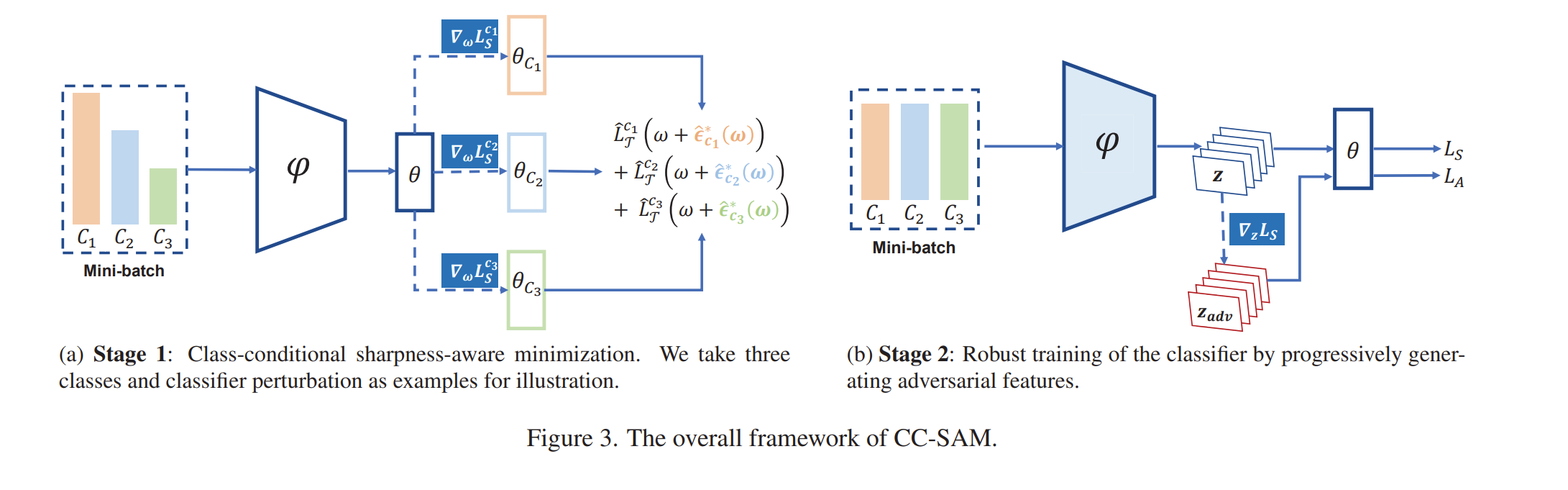
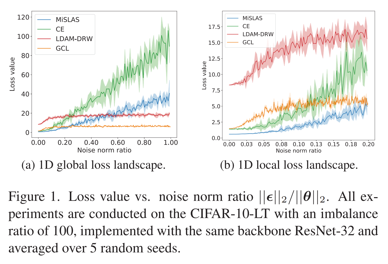
Deep Imbalanced Regression via Hierarchical Classification Adjustment

BibTex
@inproceedings{xiong2024hca,
title={Deep Imbalanced Regression via Hierarchical Classification Adjustment},
author={Xiong, Haipeng and Yao, Angela},
booktitle={Proceedings of the IEEE/CVF Conference on Computer Vision and Pattern Recognition},
year={2024}}

url= https://openaccess.thecvf.com/content/CVPR2024/papers/Xiong_Deep_Imbalanced_Regression_via_Hierarchical_Classification_Adjustment_CVPR_2024_paper.pdf
Summary

The paper proposes a method called Hierarchical Classification Adjustment (HCA) to address the issue of imbalanced regression in computer vision tasks. The approach begins by dividing the continuous target space into discrete classes or bins, which are then arranged hierarchically with progressively coarser quantization levels. The finest classifier in this hierarchy has the smallest quantization error but lower accuracy, while the coarser classifiers have higher accuracy but greater quantization errors. To balance the trade-off between classification accuracy and quantization error, the finest classifier's predictions are adjusted using predictions from the coarser classifiers. This adjustment is achieved by merging the predictions through addition and multiplication of logits, facilitated by a transition matrix that maps classes from the coarser classifiers to the finest classifier.Those transition matrix effectively duplicate the logits. Specifically, the hierarchical adjustment uses a summation or multiplication operation to merge predictions: addition-adjusted predictions are computed by summing the logits of the finest classifier with the coarser ones, while multiplication-adjusted predictions involve summing the logarithms of these logits. This coarse-to-fine merging process leverages the higher accuracy of coarse classifiers and the lower quantization error of fine classifiers to enhance the overall regression performance. Additionally, the method includes a process called Range-Preserving Distillation (HCA-d), which distills the ensemble of hierarchical classifiers into a single classifier. This distillation process ensures that the predicted ranges remain consistent across the hierarchy, addressing the inconsistency issues of standard hierarchical classification approaches. To preserve the range, the distillation process involves aligning the predictions of the hierarchical classifiers by taking the maximum value within each class range from coarser to finer classifiers, ensuring that the predicted ranges do not conflict. The distillation employs Kullback-Leibler (KL) divergence to match the probability distributions of the coarser classifiers with the finest classifier, thereby maintaining the hierarchical structure and improving the accuracy of the distilled classifier. This range-preserving adjustment is crucial for maintaining consistent predictions and efficient inference, effectively handling the challenges posed by imbalanced and insufficient data.

Problem The paper addresses the problem of performing regression tasks with imbalanced data, where using classification bins leads to a trade-off between balancing data distribution and minimizing quantization error.

Images

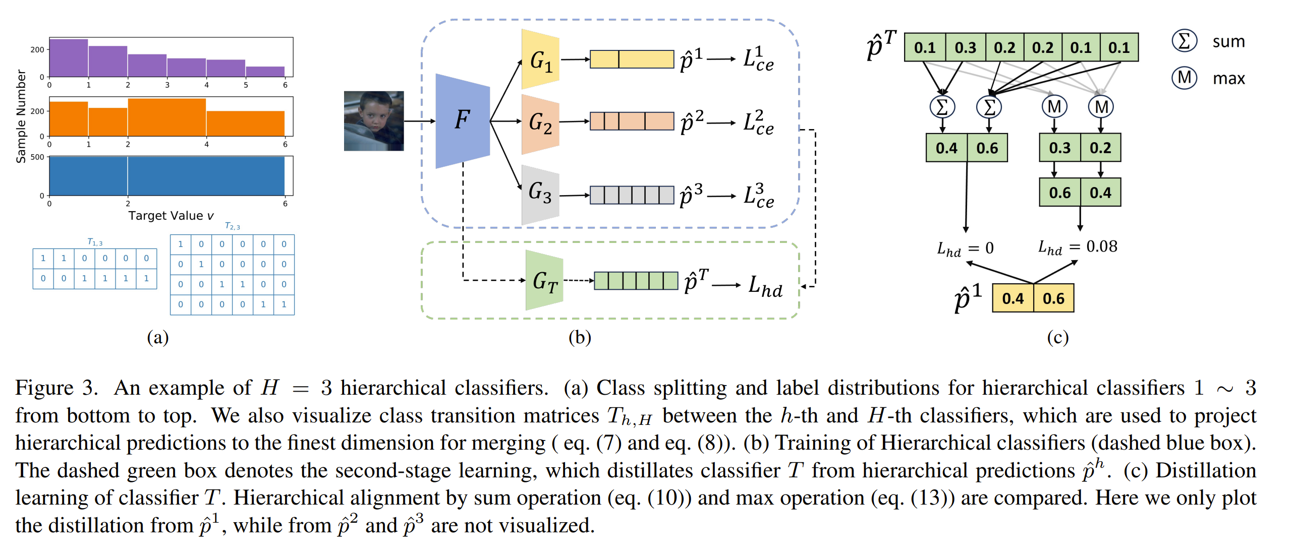
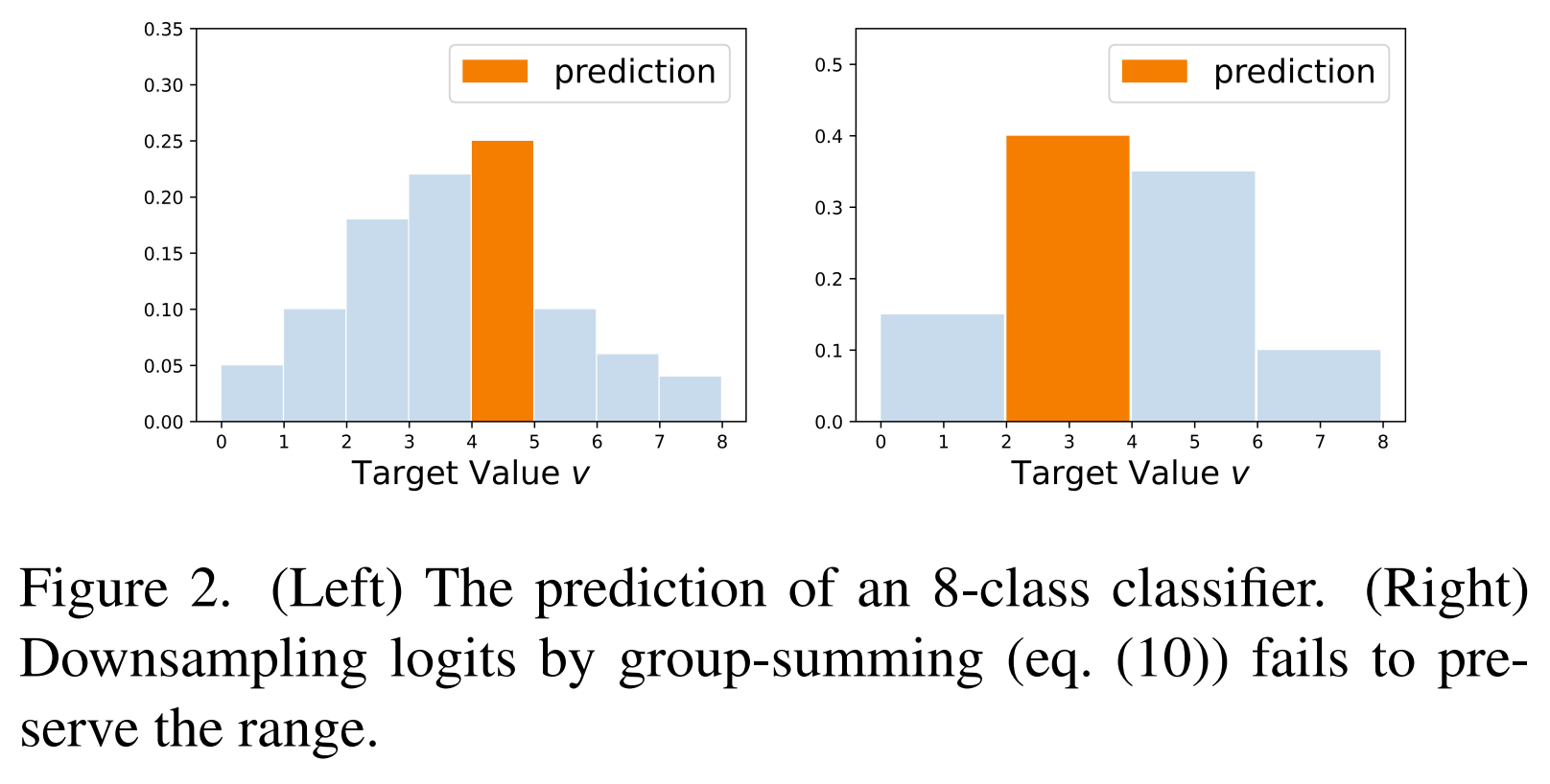
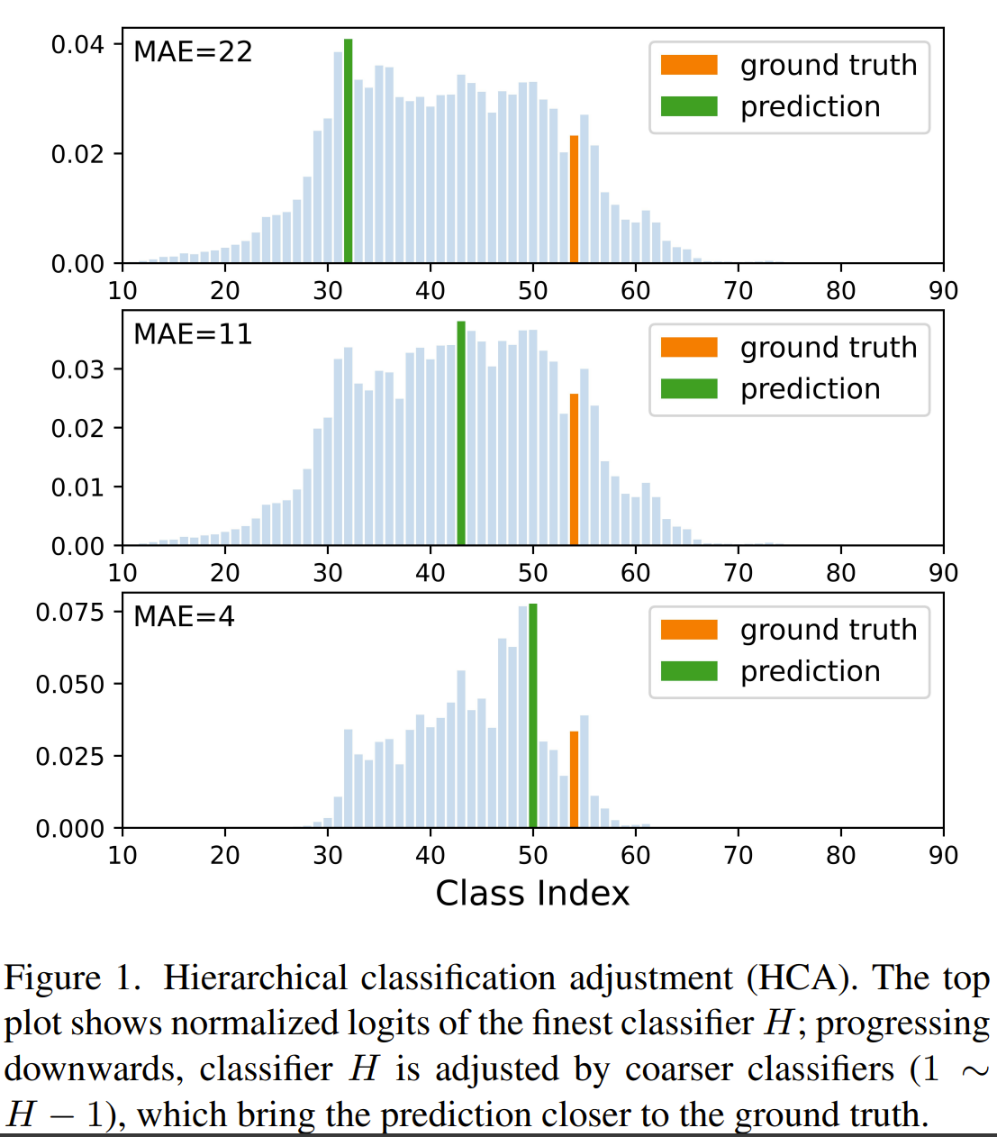
Bag of Tricks for Long-Tailed Visual Recognition with Deep Convolutional Neural Networks

BibTex
@inproceedings{zhang2021cambs,
title={Bag of tricks for long-tailed visual recognition with deep convolutional neural networks},
author={Zhang, Yongshun and Wei, Xiu-Shen and Zhou, Boyan and Wu, Jianxin},
booktitle={Proceedings of the AAAI conference on artificial intelligence},
year={2021}}

url=https://ojs.aaai.org/index.php/AAAI/article/view/16458/16265
Summary

The authors categorize the "tricks" into four main families: re-weighting, re-sampling, mixup training, and two-stage training, each containing multiple sub-methods. Re-weighting methods involve adjusting the loss function to give more importance to underrepresented classes. This includes techniques like cost-sensitive cross-entropy loss, which scales the loss inversely to the class frequency, and focal loss, which focuses more on hard-to-classify examples. However, the authors found that directly applying these re-weighting methods can sometimes lead to suboptimal performance, particularly as the number of classes increases. Re-sampling techniques aim to modify the data distribution by either over-sampling minority classes or under-sampling majority classes. Methods such as random over-sampling and random under-sampling were tested, but while they provided some improvement, they often introduced issues like overfitting or reduced data diversity. Mixup training is another approach where new training examples are created by interpolating between pairs of existing examples, which helps in regularizing the model and improving its robustness. The authors experimented with both input mixup, which operates on raw input images, and manifold mixup, which operates on intermediate feature representations within the network. Finally, in the two-stage training process, the network is first trained on the imbalanced data without any interventions, and then fine-tuned on a balanced subset using re-weighting or re-sampling methods. The authors introduce a novel method called CAM-based sampling as part of their two-stage training strategy. CAM-based sampling leverages Class Activation Maps (CAMs), which highlight the regions of an image that are most relevant to a CNN’s classification decision. The CAM-based method begins by generating these activation maps for each image in the training set using a pre-trained network. The image is then split into foreground and background regions based on the CAM values, where the foreground includes the pixels most relevant to the class label. The key idea is to apply transformations—such as flipping, rotating, or scaling—to the foreground while leaving the background unchanged. This process generates new, more informative training examples that are better suited to the network's fine-tuning process. The CAM-based approach is integrated with various re-sampling methods, creating new subsets of the data that are more balanced and discriminative. The authors found that this method significantly enhances the effectiveness of the fine-tuning process, leading to better overall performance on long-tailed datasets. In their experiments, the authors explore combinations of these tricks to identify the most effective strategy for improving long-tailed visual recognition. They discovered that combining input mixup with CAM-based balance sampling during the two-stage training process yields the best results. Specifically, in the first stage, the network is trained using input mixup, which regularizes the model by creating interpolated examples from the imbalanced data. In the second stage, the CAM-based balance sampling is employed to generate a balanced subset of the data, which the network is fine-tuned on. This combination effectively leverages the strengths of both mixup and CAM-based sampling, addressing the class imbalance issue while maintaining the robustness of the model. The authors also experimented with fine-tuning after mixup training, but they found that the best results were achieved when mixup and CAM-based sampling were applied sequentially with additional fine-tuning

Problem effectively combining and optimizing simple training "tricks" for long-tailed visual recognition tasks to improve recognition accuracy without introducing additional computational complexity.

Images

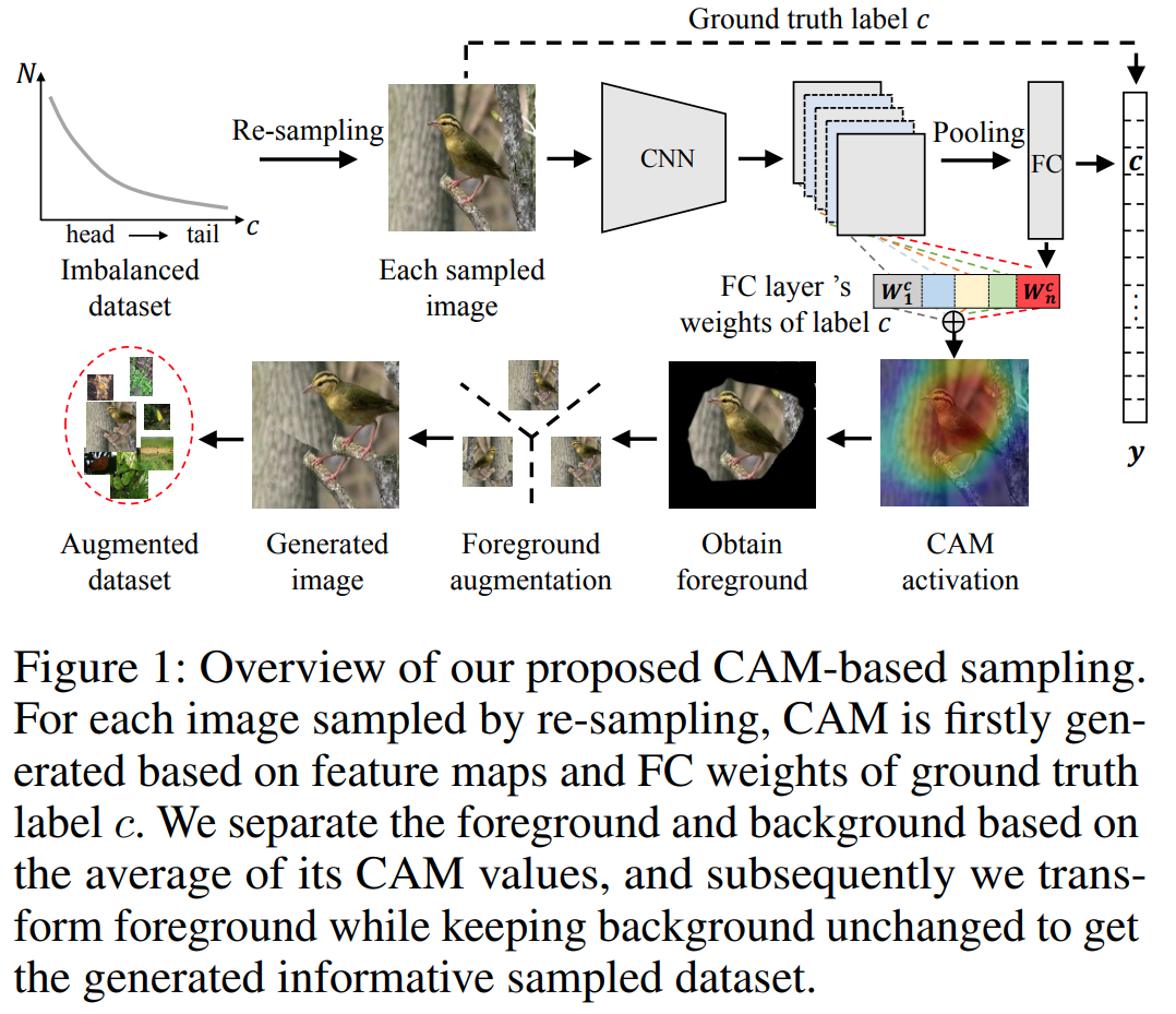
Attend and diagnose: Clinical time series analysis using attention models

BibTex
@inproceedings{song2018sand,
title={Attend and diagnose: Clinical time series analysis using attention models},
author={Song, Huan and Rajan, Deepta and Thiagarajan, Jayaraman and Spanias, Andreas},
booktitle={Proceedings of the AAAI conference on artificial intelligence},
year={2018}}

url= https://cdn.aaai.org/ojs/11635/11635-13-15163-1-2-20201228.pdf
Summary

The proposed SAnD (Simply Attend and Diagnose) architecture leverages the decoder portion of the Transformer model to process clinical time-series data without relying on the recurrence typical of RNNs. Instead, SAnD employs a masked self-attention mechanism that focuses on capturing dependencies within a single sequence of data. This design choice is particularly well-suited to the nature of clinical data, where understanding the relationships between various measurements over time is crucial. The use of positional encoding ensures that the temporal order of the data is retained, allowing the model to distinguish between different timesteps despite the lack of recurrence. A significant innovation in their approach is the dense interpolation technique, which is used to summarize multiple timestep embeddings into a smaller number of summary timesteps. This method assigns more weight to embeddings that correspond to timesteps with equivalent relative positions in the sequence, effectively capturing the central tendency of the sequence. Embeddings from timesteps that are further apart from the summary timestep are given less weight. This strategy allows the model to reduce the dimensionality of the data while preserving its essential temporal structure. However, this approach, while computationally efficient since the weights can be precomputed, has its drawbacks. The primary issue is that dense interpolation relies on a linear combination of embeddings, which may not always be semantically meaningful. A more sophisticated approach would involve learning the weights dynamically using a dense layer, which could adapt to the specific context of each timestep rather than applying a fixed linear combination. Additionally, the implementation of dense interpolation in the paper assumes that percentages are 0-indexed, while the timesteps themselves are 1-indexed, leading to an error in weight calculation that could affect the accuracy of the representation. Another challenge with dense interpolation is finding the ideal size for the summary timesteps. If the number of summary timesteps is too small, the model may not capture enough information, leading to a loss of critical temporal details. On the other hand, if the number of summary timesteps is too large, the model may suffer from the curse of dimensionality, where the data becomes too sparse and the model struggles to generalize effectively. This balance is crucial for ensuring that the dense interpolation technique provides an efficient yet accurate representation of the time-series data, enabling the model to perform well across various clinical tasks. Despite these challenges, the SAnD architecture remains a significant step forward in modeling clinical time-series data, offering a fully parallelizable and computationally efficient alternative to traditional RNN-based approaches.

Problem The paper addresses the inefficiency of RNNs in processing long clinical time-series by using attention mechanisms. However, attention can lead to high-dimensional, inefficient representations when concatenating timestep embeddings, which the authors solve by using dense interpolation.

Images

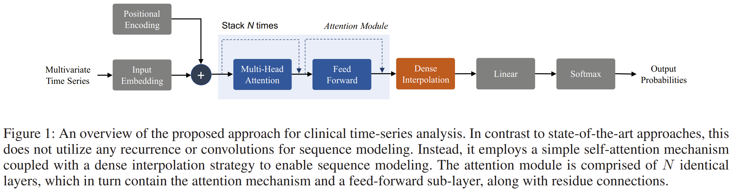
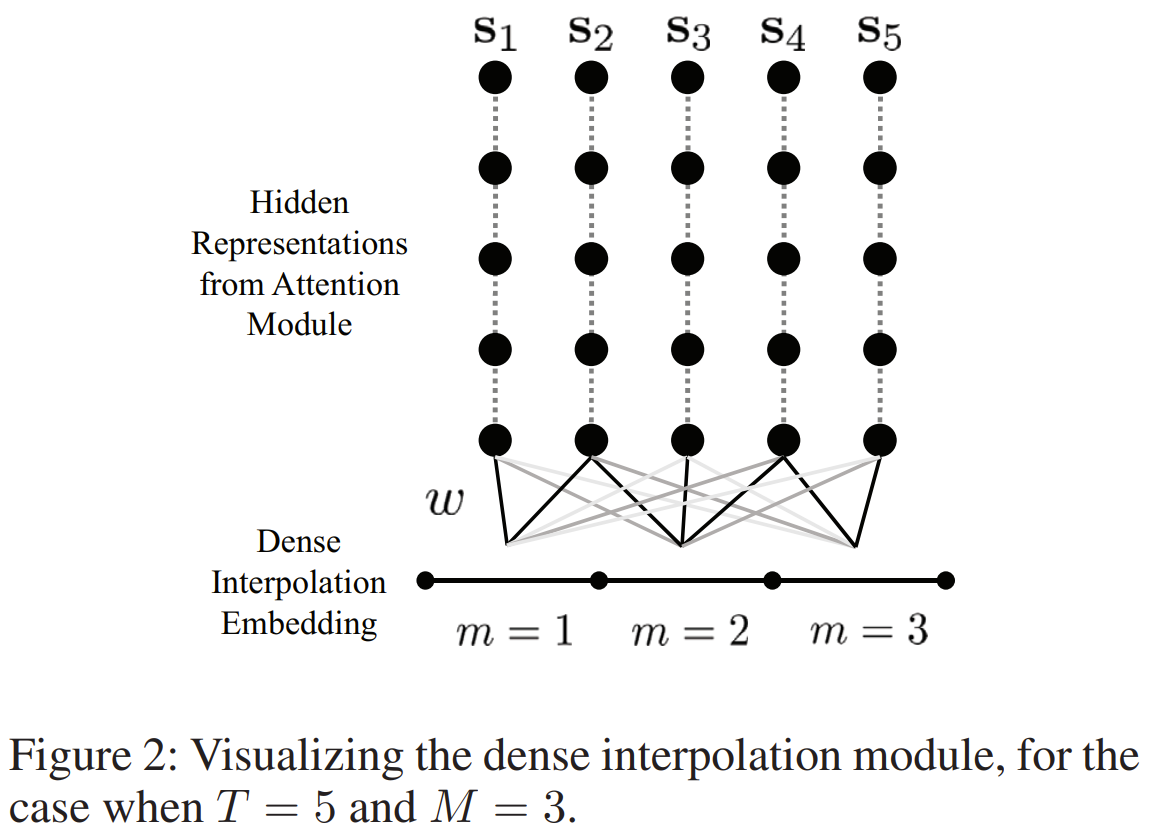
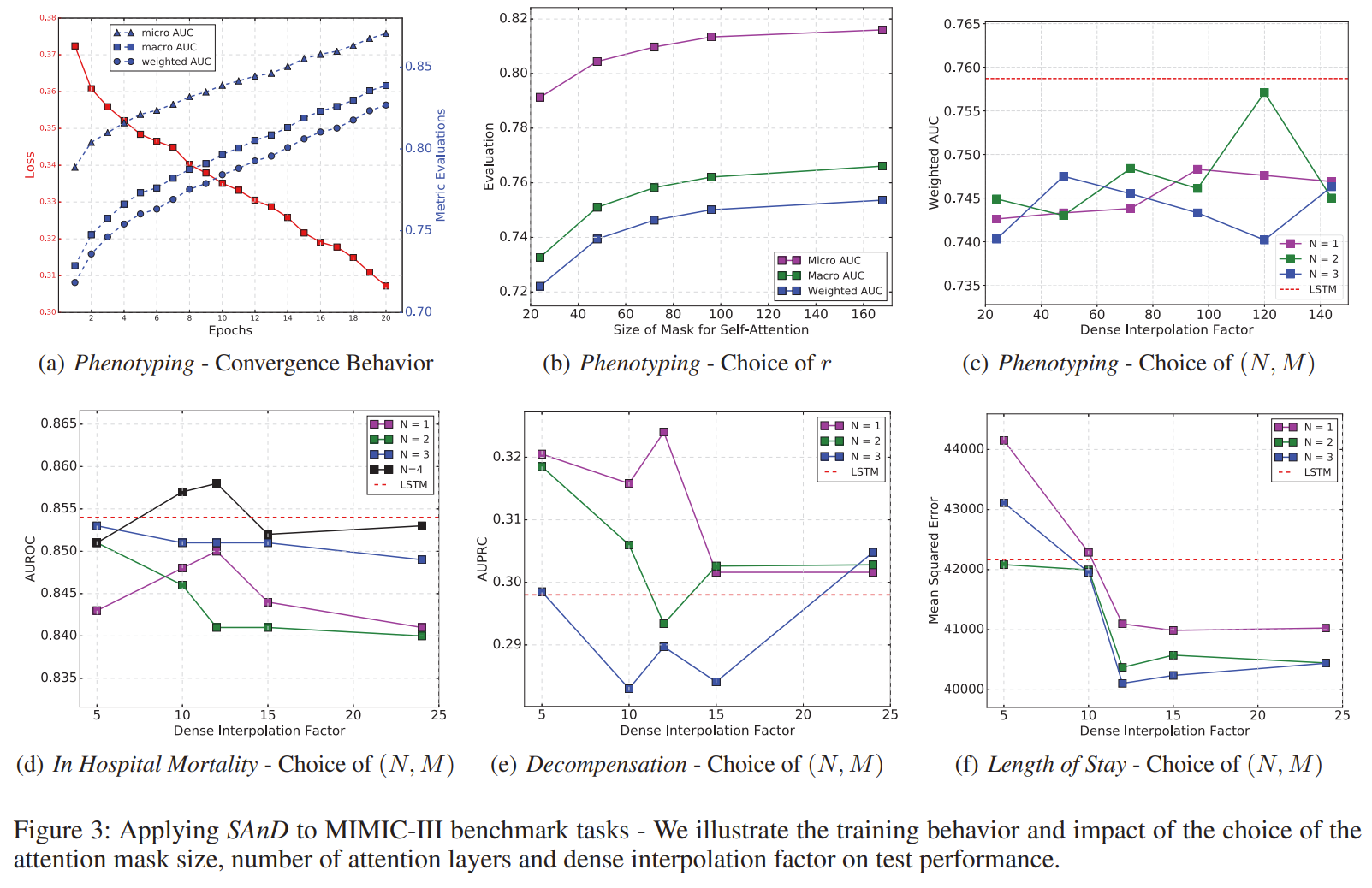
Attention-Based Autoregression for Accurate and Efficient Multivariate Time Series Forecasting

BibTex
@inproceedings{yoo2021attnar,
title={Attention-based autoregression for accurate and efficient multivariate time series forecasting},
author={Yoo, Jaemin and Kang, U},
booktitle={Proceedings of the 2021 SIAM International Conference on Data Mining (SDM)},
year={2021}}

url=https://epubs.siam.org/doi/pdf/10.1137/1.9781611976700.60
Summary

The paper introduces a novel approach called AttnAR (attention-based autoregression) for multivariate time series forecasting, addressing limitations in existing methods related to model size, complexity, and accuracy. AttnAR is designed to efficiently capture both the individual patterns within each variable and the relationships between multiple variables in a time series dataset, thereby improving forecasting performance. The AttnAR framework is built upon three main components: the Extractor Module, the Attention Module, and the Predictor Module. The Extractor Module is responsible for identifying patterns within each individual variable. It employs a mixed convolution extractor, which combines deep convolutional layers with shallow fully-connected layers. This design allows the model to capture both short-term complex patterns through the deep layers and long-term simpler patterns through the shallow layers. The use of convolutional layers helps in leveraging the temporal locality of observations, ensuring that the model can detect intricate nonlinear patterns with a minimal increase in parameters. Following the extraction of individual variable patterns, the Attention Module comes into play. This module is tasked with aggregating the extracted patterns by learning time-invariant attention maps that represent the stable correlations between different variables. The attention mechanism in AttnAR is unique in that it learns these correlations based on the intrinsic properties of the variables, rather than dynamically adjusting to the current state of the data. This is achieved through a concept called time-invariant attention, where each variable is represented by a learned embedding vector. These embeddings serve as both the query and the key in the attention mechanism, ensuring that the correlations captured are consistent and robust, regardless of changes in the input data over time. The final component, the Predictor Module, combines the variable-wise patterns and the aggregated patterns to make the final predictions. This module uses a simple multilayer perceptron (MLP) to process the concatenated patterns and produce the forecasted values. The choice of an MLP, rather than a more complex model, is intentional; the previous modules already introduce sufficient nonlinearity and complexity, so the predictor can focus on efficiently mapping the combined patterns to the predicted outputs.

Problem problem of efficient and accurate multivariate time series forecasting. Traditional models often suffer from large model sizes and poor accuracy due to their inefficiency in capturing complex intra-variable patterns and inter-variable correlations.

Images

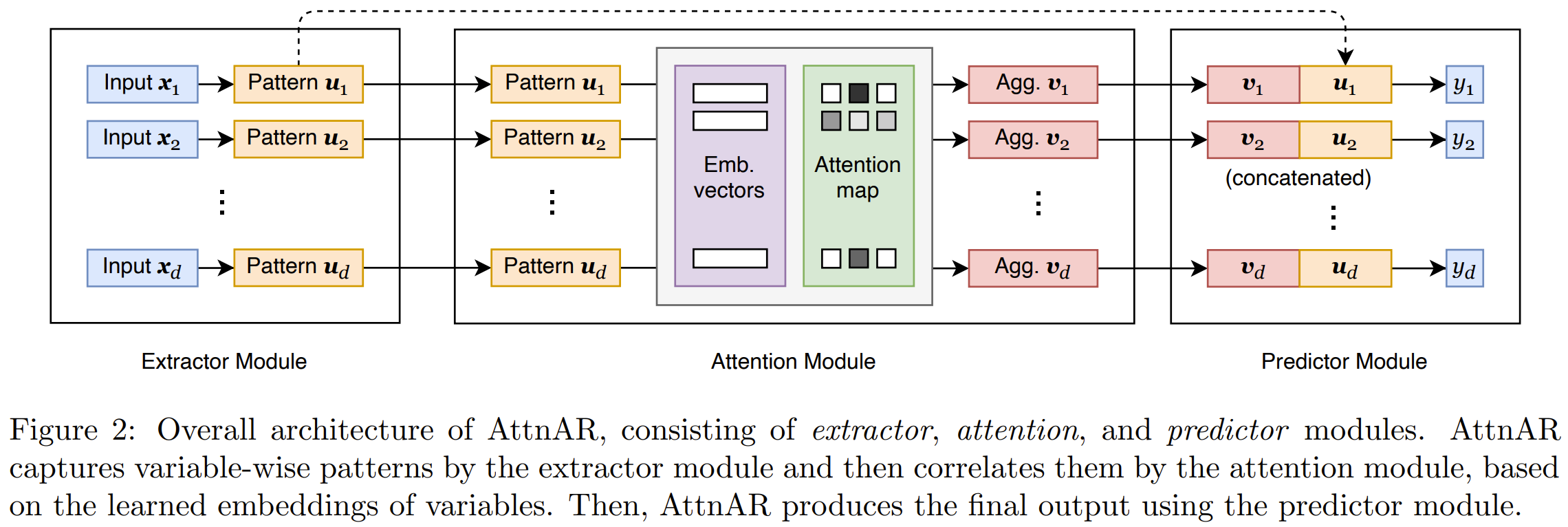
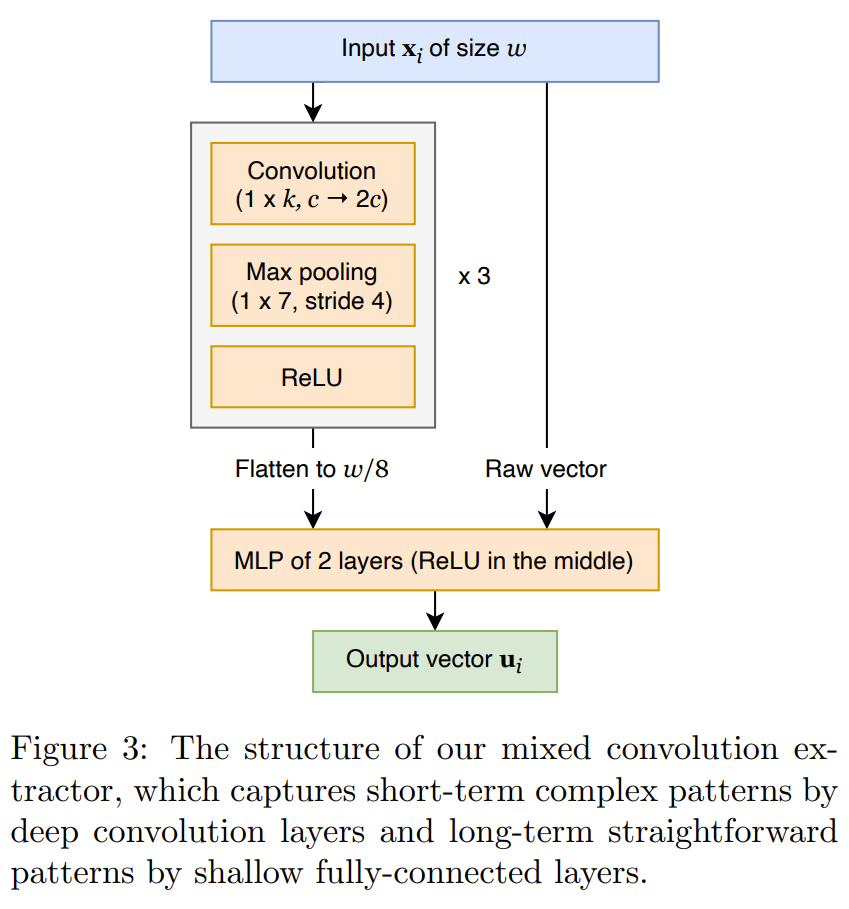
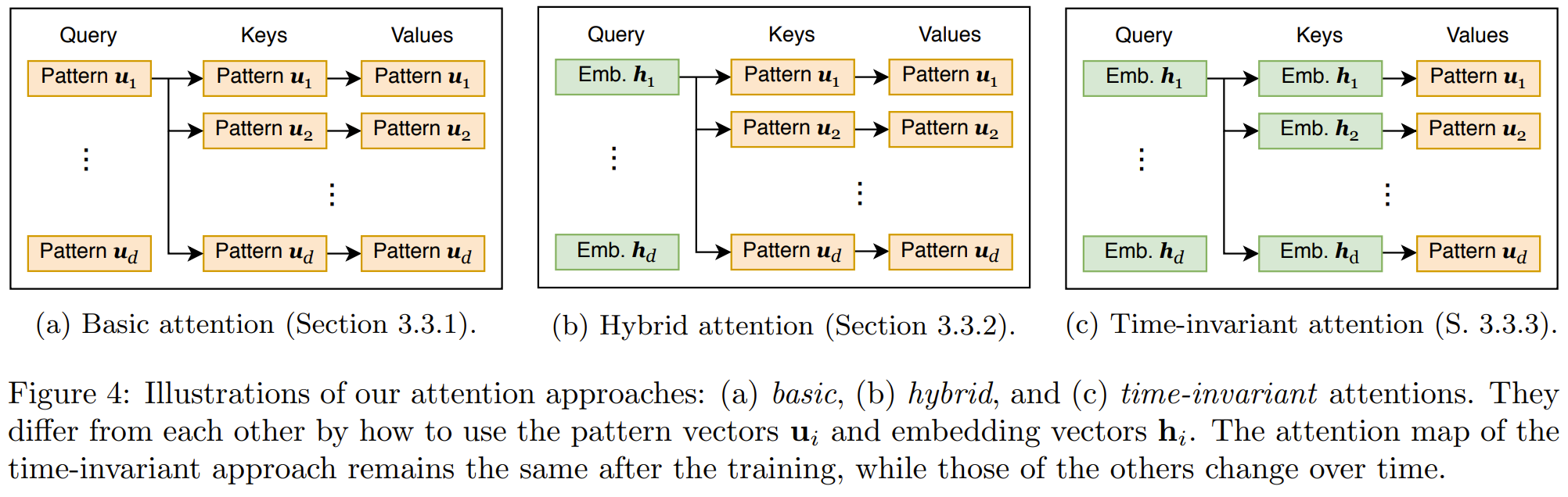
FCC: Feature Clusters Compression for Long-Tailed Visual Recognition

BibTex
@inproceedings{li2023fcc,
title={Fcc: Feature clusters compression for long-tailed visual recognition},
author={Li, Jian and Meng, Ziyao and Shi, Daqian and Song, Rui and Diao, Xiaolei and Wang, Jingwen and Xu, Hao},
booktitle={Proceedings of the IEEE/CVF conference on computer vision and pattern recognition},
year={2023}}

url= https://openaccess.thecvf.com/content/CVPR2023/papers/Li_FCC_Feature_Clusters_Compression_for_Long-Tailed_Visual_Recognition_CVPR_2023_paper.pdf
Summary

The authors propose a method called Feature Clusters Compression (FCC). The key idea behind FCC is to manipulate the feature space during the training phase to encourage the network to map features more densely. This is achieved by multiplying the original features by a scaling factor tau during training. The DNN learns the decision boundary on these scaled, or "multiplied," features, which spreads them out in the feature space. However, during testing, the original, unscaled features are used for inference. This discrepancy between the training and testing phases is what effectively compresses the feature clusters because the decision boundary learned on the multiplied features applies to the original features, pulling them closer together and reducing their spread. The authors explore four different strategies for determining the scaling factor tau. These strategies include uniform compression, where the same tau is applied to all classes; equal difference compression, where tau varies linearly across classes with larger values for majority classes and smaller values for minority classes; and two forms of half compression, where tau is applied only to the top or bottom 50% of classes by size. Equal difference compression is identified as the most effective approach because it balances the need to compress the clusters of all classes without causing excessive distortion, especially for minority classes. Minority classes, which already have features closer to decision boundaries, require smaller values of tau to avoid pushing their features across the boundary during compression. A critical aspect of the FCC method is the concept of a misclassification area, which emerges due to the difference between the features used during training (multiplied) and testing (original). As tau increases, this misclassification area grows, meaning that more features may fall into this area and be incorrectly classified. This introduces a trade-off: while higher tau values can lead to more compact clusters, they also increase the risk of misclassification. Therefore, tau must be carefully calibrated, particularly for minority classes. The FCC method not only compresses feature clusters but also tends to preserve their original shapes. However, preserving the shape of these clusters is not always beneficial because the ultimate goal should be to reshape the clusters in ways that enhance the network’s performance in downstream tasks. Additionally, the simple linear multiplier used in FCC causes the feature clusters to shift toward the bottom left of the feature space, which can be problematic for minority classes. These classes, with features already close to decision boundaries, are at greater risk of being misclassified if tau is set too high.

Problem the challenge of increasing the density of backbone feature clusters for minority classes in long-tailed visual recognition, where sparse feature clusters often lead to poor classification accuracy.

Images

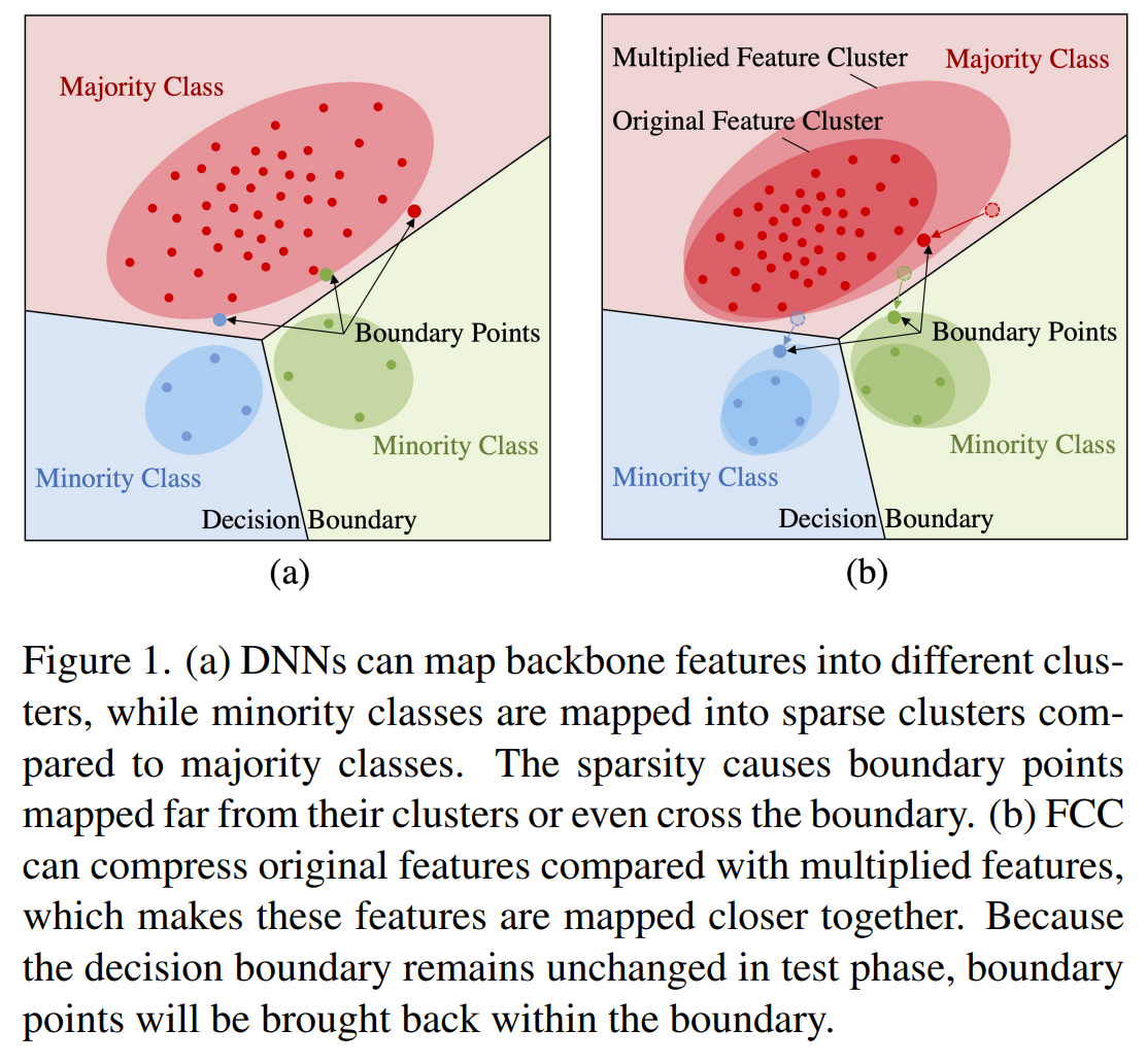
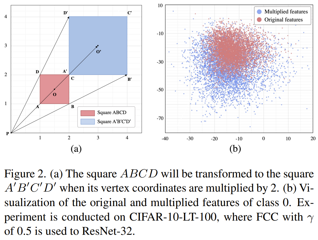
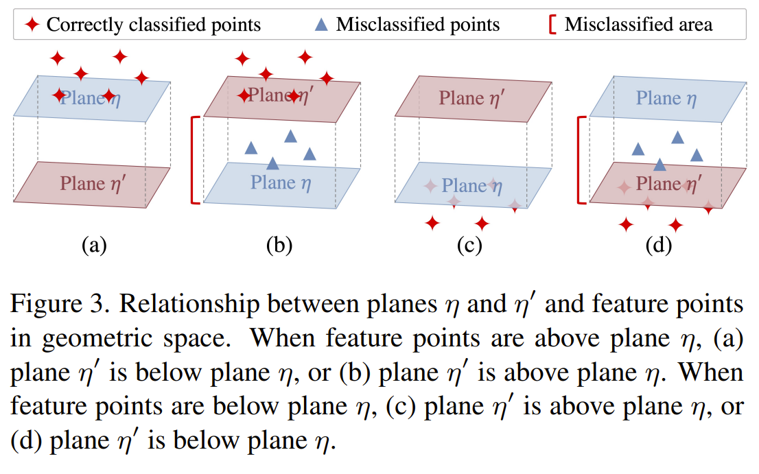
Long-Tailed Recognition by Mutual Information Maximization between Latent Features and Ground-Truth Labels

BibTex
@inproceedings{suh2023gml,
title={Long-tailed recognition by mutual information maximization between latent features and ground-truth labels},
author={Suh, Min-Kook and Seo, Seung-Woo},
booktitle={International Conference on Machine Learning},
year={2023}}

url=https://proceedings.mlr.press/v202/suh23a/suh23a.pdf
Summary

This paper addresses the problem of long-tailed recognition, where datasets have an imbalanced class distribution, leading traditional contrastive learning methods to struggle, particularly with underrepresented (tail) classes. Instead of maximizing mutual information between latent features and input instances, which doesn’t account for class imbalances, the authors propose maximizing mutual information between latent features and ground-truth labels. However, they leverage label information through class samples and class centers. While input instances are no longer the primary focus, they still act as prototypes for the classes, standing in as real samples, while the label means in the Gaussian mixture model represent idealized class centers that aren’t actual data points. This distinction allows the model to handle class imbalances while retaining the variability within each class. To ensure a balance between head and tail classes, the authors introduce class-wise queues, where head classes (with more data) have longer queues and tail classes have shorter ones. This system guarantees sufficient representation for even underrepresented classes, although the infrequent updates for tail classes can lead to outdated contrast samples. To address this, the authors employ a teacher-student framework where the teacher is pre-trained with a classification loss (Lcls). The teacher learns the class centers by optimizing the weights in its final dense layer, which encode these centers. It then produces projections (derived a few layers below the representations), and the student's task is to align its own projections with those of the teacher. The projections—not the raw representations—are used for contrastive learning, ensuring more accurate learning of class-specific features. The student is trained with both the Gaussian Mixture Likelihood (GML) loss, which models class distributions with Gaussian kernels, and the classification loss, while the teacher is trained solely with the classification loss. This dual-loss approach allows the student to learn both to classify individual samples and to model class structures in a way that balances head and tail classes effectively.

Problem The problem is how to improve contrastive learning methods for long-tailed recognition tasks by maximizing mutual information between latent features and ground-truth labels, rather than input data, to address class imbalances.

Images

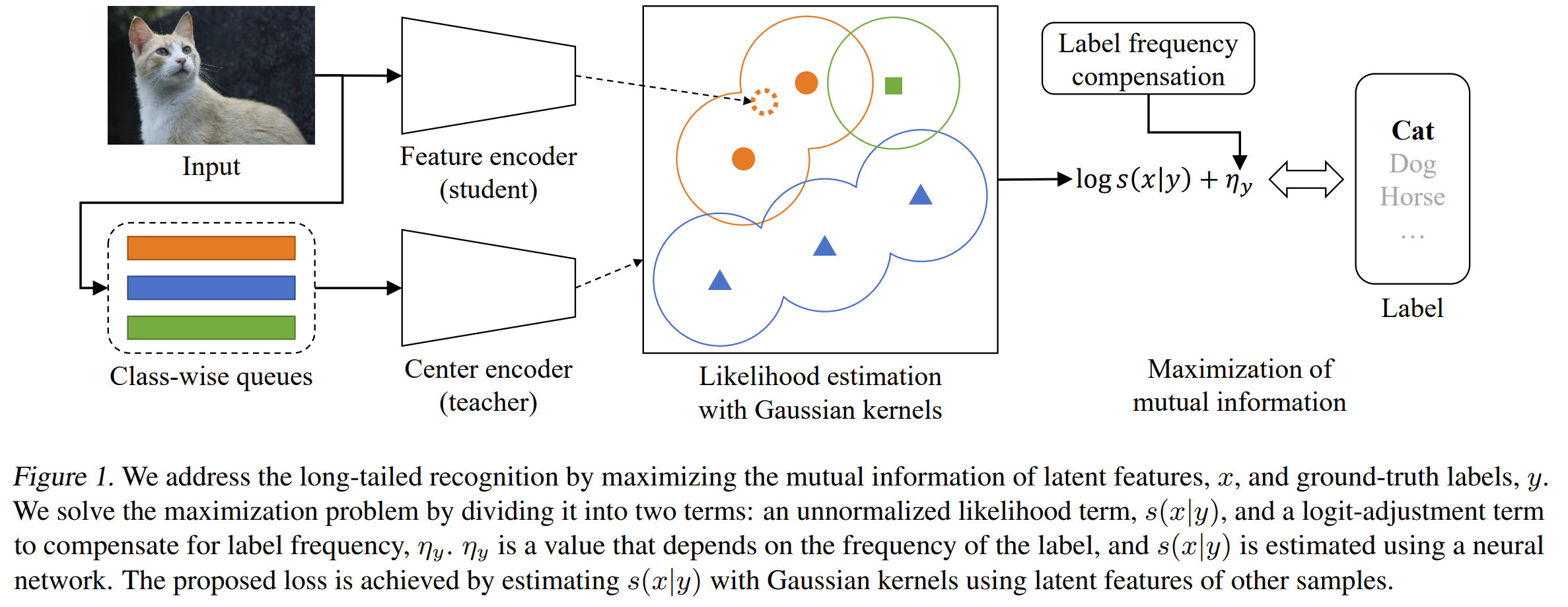
Balanced Product of Calibrated Experts for Long-Tailed Recognition

BibTex
@inproceedings{aimar2023BalPoE,
title={Balanced product of calibrated experts for long-tailed recognition},
author={Aimar, Emanuel Sanchez and Jonnarth, Arvi and Felsberg, Michael and Kuhlmann, Marco},
booktitle={Proceedings of the IEEE/CVF conference on computer vision and pattern recognition},
year={2023}}

url= https://openaccess.thecvf.com/content/CVPR2023/papers/Aimar_Balanced_Product_of_Calibrated_Experts_for_Long-Tailed_Recognition_CVPR_2023_paper
Summary

The method, called Balanced Product of Experts (BalPoE), addresses the long-tailed recognition problem by leveraging an ensemble of multiple expert models, each calibrated to handle different parts of the label distribution. The approach extends the concept of logit adjustment, a technique used to correct biases caused by imbalanced datasets, to ensembles of models. In this method, each expert is trained with a different target distribution using logit adjustment based on label frequencies. This allows the ensemble to cover both the head classes with abundant data and the tail classes with sparse data. The key idea is to combine these diverse experts such that the overall ensemble remains unbiased and consistent in minimizing the balanced error rate, which is crucial for long-tailed recognition tasks. The ensemble is formed by averaging the logits from the different experts, which are designed to target various distributions derived from the training data. During training, the method defines a set of expert models, each with a specific bias parameterization. By adjusting the logits for each expert according to a different target distribution, the method ensures that each expert specializes in a particular region of the class distribution, balancing the effect of the long-tailed distribution. To achieve an overall unbiased prediction from the ensemble, the paper derives a theoretical framework showing that if the average bias across all experts equals zero, the ensemble prediction is Fisher-consistent, meaning it is optimal for minimizing balanced error. A critical component of this approach is ensuring that each expert model is well-calibrated. Calibration refers to the model's ability to provide accurate probability estimates, which is essential for the proper functioning of the logit adjustment. The method uses mixup, a data augmentation technique, to improve the calibration of individual experts. Mixup generates new training samples by interpolating between pairs of examples and their labels, which helps the model avoid overconfidence and improves the generalization to tail classes. Importantly, mixup does not alter the underlying label distribution, making it compatible with the logit adjustment framework. This calibration step ensures that the ensemble remains unbiased and effective in handling the varying distributions encountered during training and inference. The mixup is of both features and labels with U-shape sampling, closer to the extreme ends. During inference, the method combines the outputs of all the experts by averaging their adjusted logits before applying the softmax function to produce the final prediction. This process allows the ensemble to leverage the strengths of each expert and generate more robust predictions across the entire class distribution. The ensemble's ability to generalize over different distributions enables it to perform well on imbalanced datasets, particularly in scenarios where the test distribution differs from the training distribution.

Problem The paper tackles the challenge of learning unbiased and effective representations in long-tailed recognition tasks, where the label distribution is highly imbalanced, by addressing the difficulty of generalizing well over classes with limited data.

Images

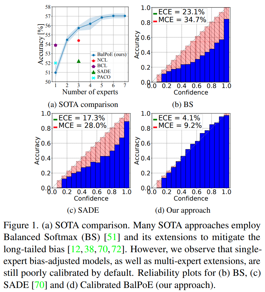
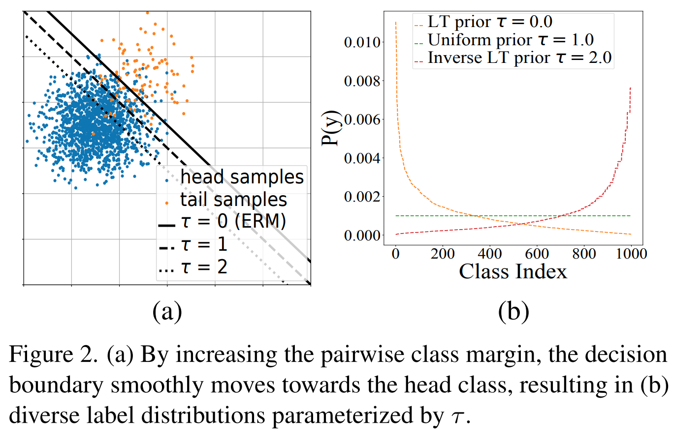
DeiT-LT: Distillation Strikes Back for Vision Transformer Training on Long-Tailed Datasets

BibTex
@inproceedings{rangwani2024deitlt,
title={DeiT-LT: Distillation Strikes Back for Vision Transformer Training on Long-Tailed Datasets},
author={Rangwani, Harsh and Mondal, Pradipto and Mishra, Mayank and Asokan, Ashish Ramayee and Babu, R Venkatesh},
booktitle={Proceedings of the IEEE/CVF Conference on Computer Vision and Pattern Recognition},
year={2024}}

url= https://openaccess.thecvf.com/content/CVPR2024/papers/Rangwani_DeiT-LT_Distillation_Strikes_Back_for_Vision_Transformer_Training_on_Long-Tailed_CVPR_2024_paper.pdf
Summary

The proposed method, DeiT-LT (Data-efficient Image Transformer for Long-Tailed Data), enhances Vision Transformer (ViT) training for long-tailed datasets by introducing key improvements centered around distillation from CNNs. The architecture of DeiT-LT is based on the Vision Transformer, which processes input images by splitting them into patches and passing them through a sequence of self-attention blocks. To address the challenge of imbalanced data, DeiT-LT incorporates both a classification (CLS) token, which focuses on majority (head) classes, and a distillation (DIST) token, which becomes specialized in handling minority (tail) classes. A central idea in DeiT-LT is to distill knowledge from CNNs to ViTs using a strategy of Out-of-Distribution (OOD) images. Unlike the standard DeiT model, where distillation occurs from a CNN pre-trained on large datasets, DeiT-LT generates OOD images by applying strong data augmentations. These augmented images are typically "out of distribution" for the CNN teacher (which may have lower accuracy on these images), yet this helps the ViT student network generalize better. By training on OOD images, the DIST token in DeiT-LT learns CNN-like local features in early blocks, which improves generalization for tail classes. This divergence in training between the CLS and DIST tokens allows DeiT-LT to effectively handle both head and tail classes within a single architecture. DeiT-LT also introduces the use of Sharpness-Aware Minimization (SAM) to train the CNN teachers. SAM leads to "flat" minima, which encourage the learning of low-rank, generalizable features. These low-rank features are then distilled into the ViT, enabling the model to handle the inherent imbalance in the dataset. The low-rank nature of the features ensures better generalization across ViT blocks, further improving performance on minority classes. The method also incorporates Deferred Re-Weighting (DRW) for the distillation loss. In DRW, the loss assigned to each class is dynamically adjusted based on its frequency in the dataset, with greater emphasis placed on tail classes as training progresses. This step further focuses the DIST token’s attention on tail classes, while the CLS token remains an expert on head classes. Importantly, this approach enables the training of distinct experts (CLS for head classes and DIST for tail classes) within a single ViT backbone without the need for multiple expert models, reducing the complexity at inference time. Finally, DeiT-LT maintains computational efficiency by using small CNN models (e.g., ResNet-32) for distillation rather than larger models (e.g., RegNetY-16GF), significantly reducing training time while still achieving high performance. The combination of OOD distillation, SAM-trained teachers, and DRW creates a robust method for training Vision Transformers on long-tailed datasets, addressing both data imbalance and overfitting to majority classes.

Problem The paper addresses the challenge of training Vision Transformers on long-tailed datasets by introducing a distillation approach from CNNs to improve performance on minority (tail) classes without sacrificing accuracy on majority (head) classes.

Images

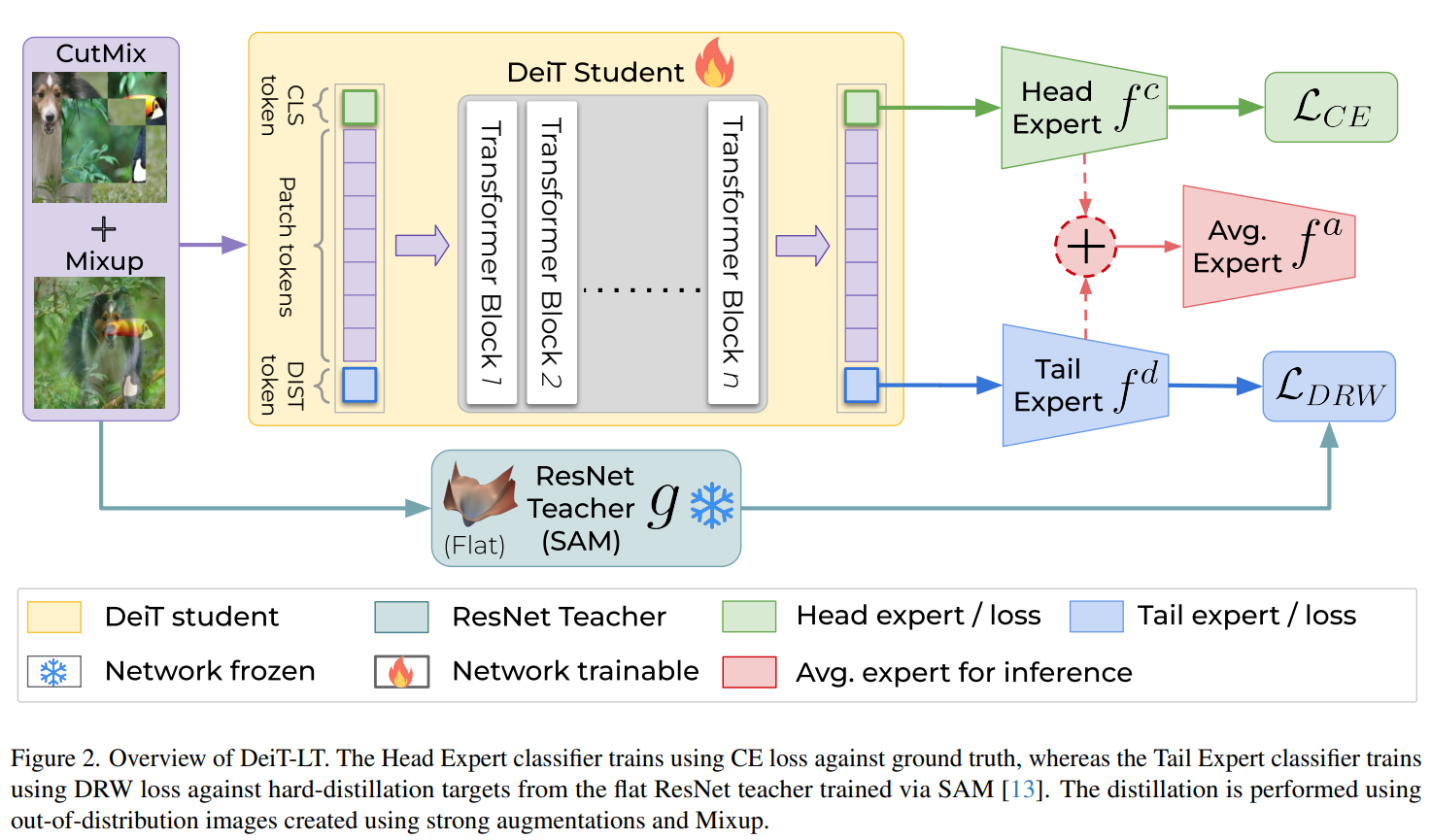
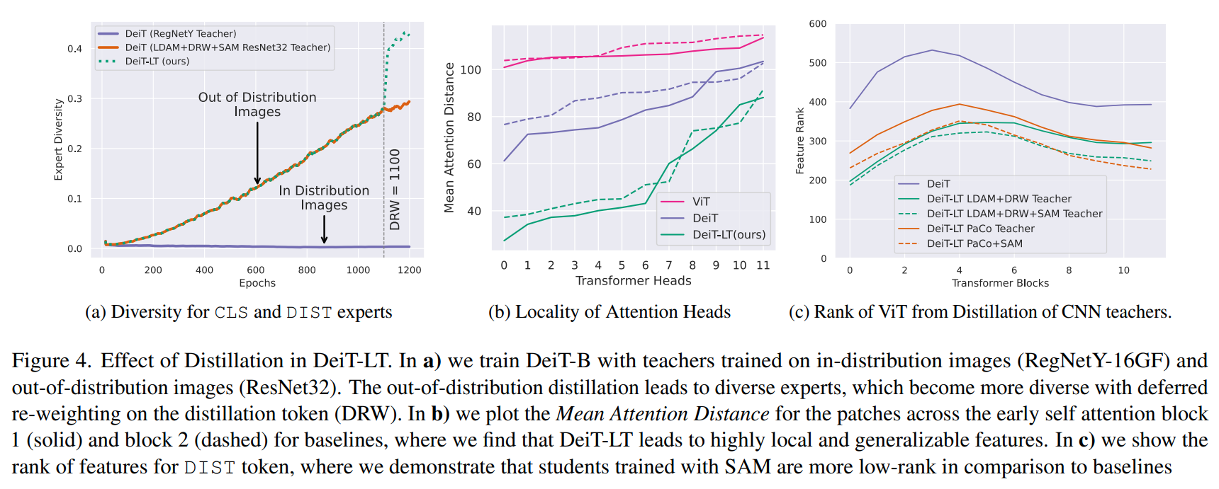
No one left behind: Improving the worst categories in long-tailed learning

BibTex
@inproceedings{du2023cegml,
title={No one left behind: Improving the worst categories in long-tailed learning},
author={Du, Yingxiao and Wu, Jianxin},
booktitle={Proceedings of the IEEE/CVF conference on computer vision and pattern recognition},
year={2023}}

url= https://openaccess.thecvf.com/content/CVPR2023/papers/Du_No_One_Left_Behind_Improving_the_Worst_Categories_in_Long-Tailed_CVPR_2023_paper.pdf
Summary

This paper addresses the issue of low recall for worst-performing categories in long-tailed image classification. The authors propose a novel method called Geometric Mean Loss (GML) to improve the performance of these categories without sacrificing overall accuracy. GML is designed as a plug-in method that can be applied to various existing long-tailed recognition approaches. The authors argue that harmonic mean of per-class recall is a better objective than arithmetic mean for long-tailed recognition, as it's more sensitive to low values and thus encourages improvement of the worst-performing classes. However, since harmonic mean is difficult to optimize directly due to its use of reciprocals, they propose using geometric mean as a surrogate objective. The geometric mean serves as a middle ground between arithmetic and harmonic means in terms of sensitivity to low values, aligning with their goal of ensuring "no category is left behind" in long-tailed recognition tasks. The core idea of GML is to maximize the geometric mean of per-class recall. The GML loss is defined as the negative log of the average softmax outputs for each class. It incorporates a re-weighting scheme similar to balanced softmax cross-entropy. The method consists of three stages: pre-training using an existing method, fine-tuning the classifier with the GML loss while freezing the backbone, and an optional ensemble stage. During the fine-tuning stage, only the classifier is re-trained while the backbone remains frozen. This approach allows the method to be easily integrated with existing techniques. The optional ensemble stage combines predictions from both the original and fine-tuned classifiers. It uses temperature scaling for calibration, introducing two hyperparameters: t_old and t_new. These temperatures are applied to the logits of the original and fine-tuned classifiers, respectively, before combining their predictions through simple averaging. Ablation studies revealed several important aspects of the method. The re-weighting scheme in GML was found to be crucial for performance, outperforming alternatives like re-sampling. The ensemble stage's effectiveness was explored through different temperature combinations, showing that preserving more information from the fine-tuned classifier (lower t_new) was important for improving the lowest recall. The authors also demonstrated that while GML can be used to train a model from scratch, it performs best when applied as a fine-tuning step to existing methods. This approach provides a simple yet effective way to address the problem of low recall in worst-performing categories in long-tailed recognition, ensuring that no category is left behind while maintaining high overall accuracy.

Problem The true problem identified is that existing long-tailed recognition methods often result in very low recall (close to zero) for some of the worst-performing categories, even as overall accuracy improves. The authors argue this means some categories are essentially "left behind" or ignored by current approaches.

Images

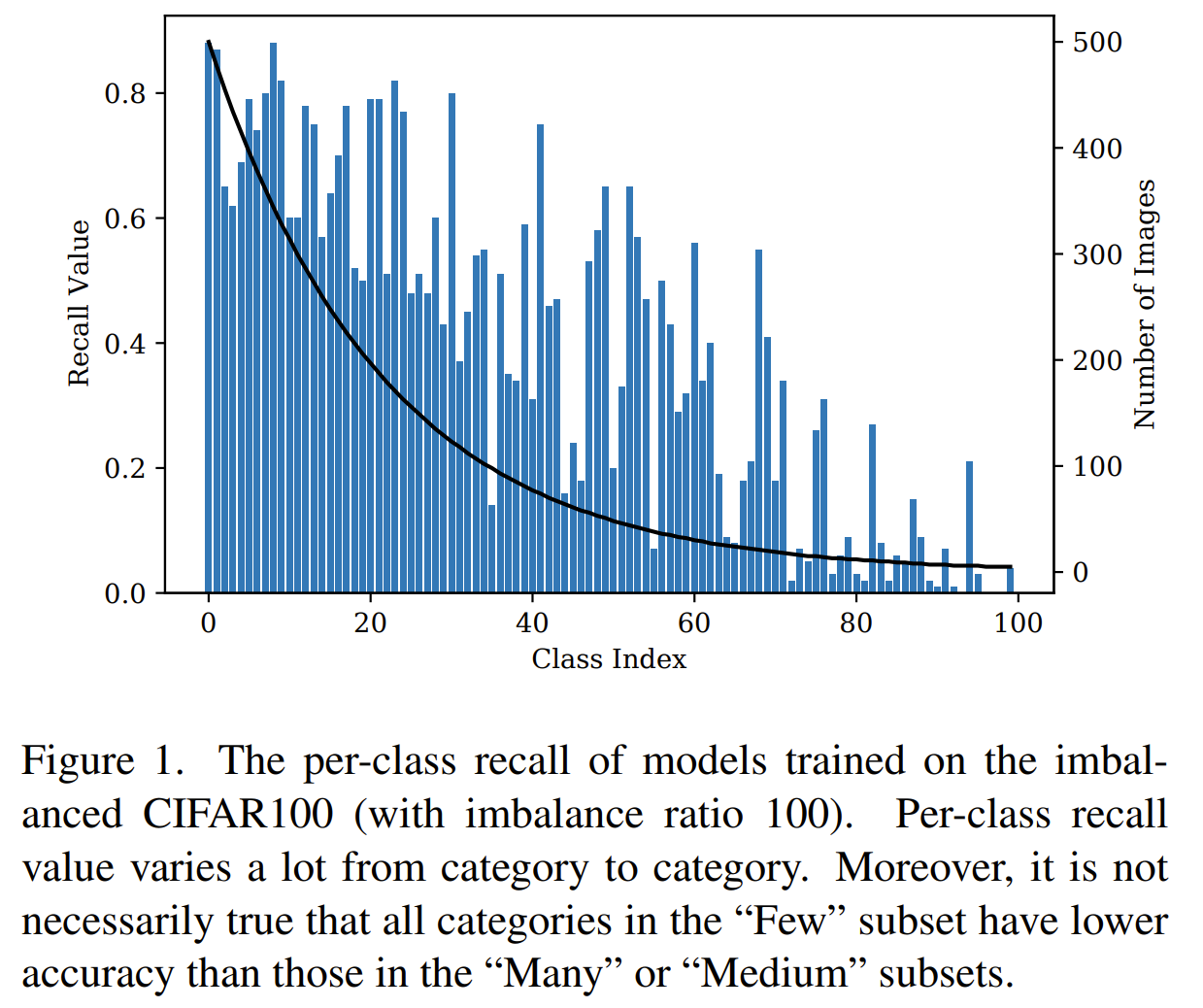
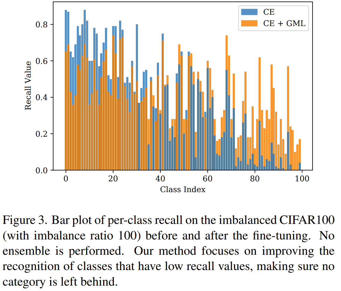
Curvature-Balanced Feature Manifold Learning for Long-Tailed Classification

BibTex
@inproceedings{ma2023cr,
title={Curvature-balanced feature manifold learning for long-tailed classification},
author={Ma, Yanbiao and Jiao, Licheng and Liu, Fang and Yang, Shuyuan and Liu, Xu and Li, Lingling},
booktitle={Proceedings of the IEEE/CVF conference on computer vision and pattern recognition},
year={2023}}

url= https://openaccess.thecvf.com/content/CVPR2023/papers/Ma_Curvature-Balanced_Feature_Manifold_Learning_for_Long-Tailed_Classification_CVPR_2023_paper.pdf
Summary

The paper first establishes a systematic way to measure geometric characteristics of perceptual manifolds (feature spaces) in deep neural networks. They propose methods to calculate the volume of these manifolds, the degree of separation between different manifolds, and most importantly, the curvature of these manifolds using neighboring points. For calculating manifold volume, they introduce a method using the determinant of the covariance matrix of features, with special consideration for non-full rank cases by adding an identity matrix. To measure separation between manifolds, they develop an asymmetric measure that accounts for different manifold volumes, ensuring that when manifolds overlap, the impact on smaller manifolds is appropriately weighted more heavily. The curvature calculation is particularly sophisticated. For each point in the manifold, they first estimate the normal vector using neighboring points through eigenvalue decomposition of the local covariance matrix. They then project neighboring points onto the tangent space and fit a quadratic hypersurface to estimate the Gauss curvature. This process is done for all points, and the average is taken as the manifold's complexity measure. Their key methodological contribution is the Curvature Regularization (CR) term. This regularization aims to balance curvature across all class manifolds while encouraging overall flatter manifolds. The CR term is designed with three principles: stronger penalties for higher curvature manifolds, equal penalties when curvatures are balanced, and an overall tendency to decrease total curvature. The final loss function combines the original loss with the CR term, weighted by a logarithmic function of the training epoch. To make this practical in training, they introduce Dynamic Curvature Regularization (DCR). DCR maintains a first-in-first-out storage pool of recent feature embeddings, addressing the challenge of calculating manifold properties without access to all features at once. This approach leverages the observation that features drift slowly during training, making recent historical features useful for curvature estimation. The storage pool is updated continuously during training, with the oldest batch being replaced by the newest one at each iteration. The implementation requires careful hyperparameter selection, particularly for τ, which controls the relative weight of the curvature regularization term. The authors find that different dataset sizes require different τ values, with larger datasets needing larger values to allow more time for proper feature separation. The method can be integrated with any existing loss function and training framework, requiring only the addition of the feature storage pool and curvature calculation components.

Problem The paper solves the problem that class accuracy in deep learning becomes increasingly negatively correlated with feature manifold curvature during training, while existing methods only focus on feature separability and ignore this curvature imbalance issue.

Images

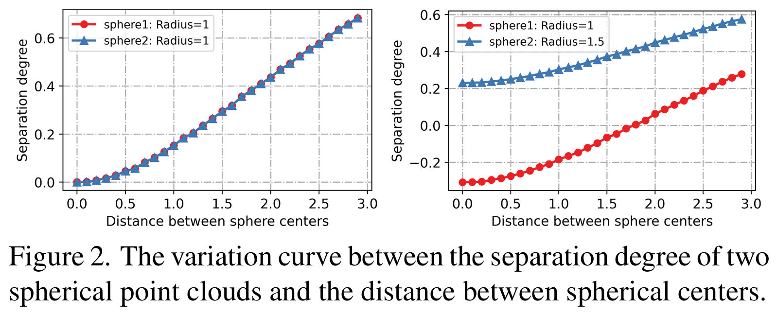
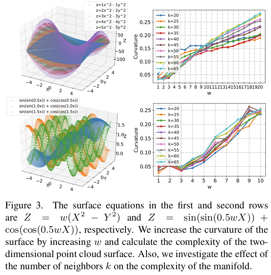
Superdisco: Super-class discovery improves visual recognition for the long-tail

BibTex
@inproceedings{du2023superdisco,
title={Superdisco: Super-class discovery improves visual recognition for the long-tail},
author={Du, Yingjun and Shen, Jiayi and Zhen, Xiantong and Snoek, Cees GM},
booktitle={Proceedings of the IEEE/CVF Conference on Computer Vision and Pattern Recognition},
year={2023}}

url= https://openaccess.thecvf.com/content/CVPR2023/papers/Du_SuperDisco_Super-Class_Discovery_Improves_Visual_Recognition_for_the_Long-Tail_CVPR_2023_paper.pdf
Summary

The paper introduces SuperDisco, an algorithm that learns to discover semantic super-class representations to help with long-tailed visual recognition. The key insight comes from how humans effortlessly handle object recognition from rarely seen classes by using different levels of semantic abstraction. The authors note that while individual classes may have imbalanced distributions (many examples of common objects, few of rare ones), their corresponding super-classes tend to be more balanced. For example, while specific car models may be rare in a dataset, the overall super-class of "vehicles" maintains a good number of examples due to the shared visual features among vehicles, enabling knowledge transfer from frequent to rare classes. SuperDisco constructs a hierarchy of graphs that work together to refine features. The super-class graph (C) discovers and represents semantic groupings through learnable vertices (representing super-classes) and edges (representing relationships between super-classes). The relationship graph (R) connects original image represenations to the super-class graph by computing similarities, allowing features to be refined through message passing with relevant super-classes. To improve robustness, Meta-SuperDisco introduces a prototype graph (P) built from a small balanced dataset to capture clean sample-level relationships. Finally, a super graph (S) connects the prototype graph to the super-class graph (C), allowing the prototypes to guide better super-class discovery Interestingly, the authors structure their super-class hierarchy to start with fewer classes at higher levels and progressively increase the number of classes at lower levels (e.g., 2->4->8->16). This is counter to traditional deep learning architectures where feature representations typically start large and get progressively smaller. Through message passing mechanisms across these interconnected graphs, the original image features are refined by attending to relevant super-class representations. This helps pull tail class features away from being dominated by head class features, making them more discriminative. The deeper and wider graph structures are particularly important when dealing with severe class imbalance, as they allow the model to discover more nuanced hierarchical relationships. The paper's significance lies in its novel approach to automatically discovering and utilizing semantic hierarchies without requiring explicit super-class labels, effectively mimicking humans' intuitive ability to use abstract categorization for recognizing rare objects. This differs from previous approaches that either required predefined hierarchical labels or focused on rebalancing techniques without considering semantic relationships.

Problem Current AI image classifiers lack humans' natural ability to leverage different levels of semantic abstraction (like grouping objects into higher-level categories) to effectively recognize objects from rarely seen classes.

Images

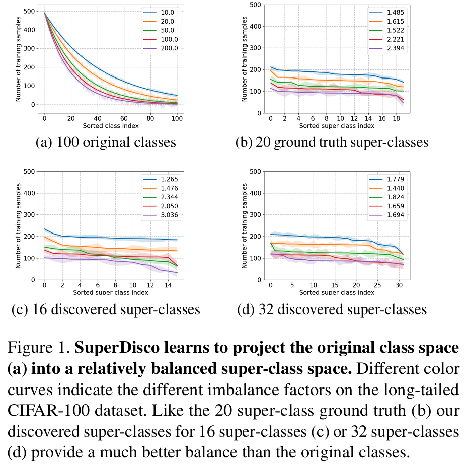
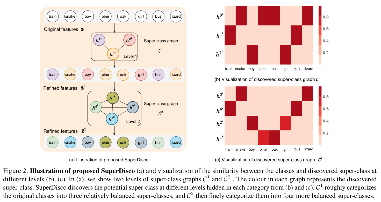
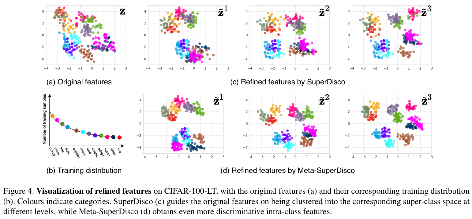
Enhancing Class-Imbalanced Learning with Pre-Trained Guidance through Class-Conditional Knowledge Distillation

BibTex
@inproceedings{li2024acckd,
title={Enhancing Class-Imbalanced Learning with Pre-Trained Guidance through Class-Conditional Knowledge Distillation},
author={Li, Lan and Li, Xin-Chun and Ye, Han-Jia and Zhan, De-Chuan},
booktitle={Forty-first International Conference on Machine Learning}
}

url=https://openreview.net/pdf?id=O4nXWHPl6g
Summary

The paper introduces a method to address the challenges of class-imbalanced learning (CIL) by leveraging the capabilities of large-scale pre-trained models to enhance the generalization of features, particularly for minority classes. Central to the proposed approach is the concept of Class-Conditional Knowledge Distillation (CCKD), which departs from conventional knowledge distillation techniques by focusing on learning the teacher model's class-conditional probability distribution p(x|y). This shift is crucial because traditional methods transfer the posterior distribution p(y|x), which often fails to generalize well on imbalanced datasets due to insufficient representation of minority classes. To implement CCKD, the student model learns the class-conditional probability distribution p(x|y) by normalizing the teacher model's predictions p(y|x) with the class priors, which are computed based on Bayes' theorem. However, since the continuous nature of x makes direct optimization infeasible, the method employs a reformulation that indirectly learns p(x|y) through adjusted distillation loss functions. The model integrates these probabilities with logit adjustments to counteract the imbalanced class distributions. The method is extended with Augmented Class-Conditional Knowledge Distillation (ACCKD), which further improves generalization by introducing a synthetic class-balanced dataset generated using data augmentation techniques like Mixup and CutMix. These methods create new training samples by interpolating or combining samples from different classes. By ensuring a balanced distribution of classes in the synthetic dataset, the approach helps the student model learn a more generalized p(x|y). Additionally, a feature imitation loss is introduced to align the feature spaces of the teacher and student models, promoting the transfer of intrinsic feature structures across the two models. This alignment is achieved by minimizing the cosine distance between the feature embeddings from the teacher and student networks. While the proposed method introduces novel and effective techniques for addressing class imbalance, a few issues remain with the paper. Notably, the authors conflate the use of likelihood p(x|y) and posterior p(y|x) terms, treating them interchangeably in several contexts, which may lead to theoretical ambiguities and potential misunderstandings. This conflation undermines the conceptual clarity of the proposed approach and makes it challenging to rigorously assess its implications. Addressing such issues would strengthen the paper's contributions and solidify its impact on the field.

Problem This paper addresses the problem of improving class-imbalanced learning by leveraging pre-trained models to enhance the generalization of features for minority classes through class-conditional knowledge distillation and data augmentation techniques.

Images

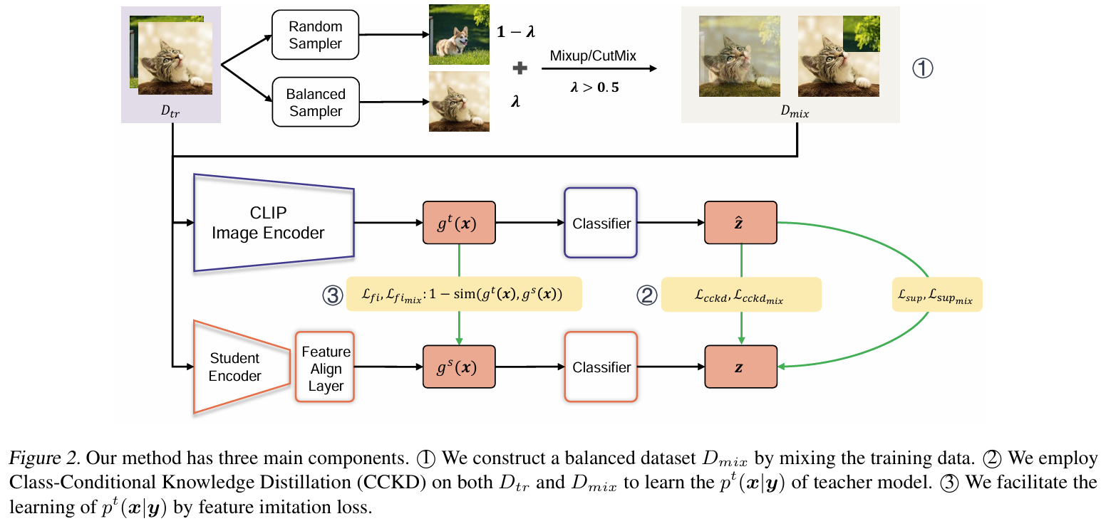
Distribution alignment optimization through neural collapse for long-tailed classification

BibTex
@inproceedings{gao2024disA,
title={Distribution alignment optimization through neural collapse for long-tailed classification},
author={Gao, Jintong and Zhao, He and dan Guo, Dan and Zha, Hongyuan},
booktitle={Forty-first International Conference on Machine Learning},
year={2024}}

url=https://openreview.net/pdf?id=Hjwx3H6Vci
Summary

The paper proposes a novel method, Distribution Alignment Optimization (DisA), to address the challenges of long-tailed classification, where class imbalance results in poor representation quality for minority classes. The method leverages two foundational concepts: Neural Collapse (NC) and Optimal Transport (OT). Neural Collapse is a phenomenon observed during training on balanced datasets where, in the final phase, last-layer features collapse into their within-class means. These means, along with the classifier weight vectors, align into a geometric structure called the simplex Equiangular Tight Frame (ETF), which ensures that classes are optimally separated in representation space. However, on imbalanced datasets, achieving NC is challenging because the minority class representations do not align well with the ideal ETF structure, leading to performance degradation. Optimal Transport, a mathematical framework originating from the problem of moving distributions efficiently, is the second key concept underlying DisA. OT finds the minimal cost of transforming one probability distribution into another, where the cost is defined by a chosen distance metric, such as cosine distance. Two important components of OT are the cost matrix and the transport plan. The cost matrix quantifies the distance between individual elements of two distributions, and the transport plan determines how much mass should be moved from each element of the source distribution to the target distribution to minimize the overall cost. By minimizing this transport cost, OT provides a principled way to align distributions in a way that respects their underlying geometry. In DisA, the last-layer representations of the model are treated as the source distribution P, which is imbalanced due to the long-tailed nature of the data. The target distribution Q is defined by the balanced ETF structure, which represents the ideal configuration for class separation. DisA minimizes the OT distance between P and Q, aligning the imbalanced representations with the balanced ideal. This alignment is achieved through entropy-regularized OT, which makes the optimization computationally efficient while preserving the interpretability of the transport plan. The regularization ensures smooth alignment by discouraging overly sharp or rigid transport assignments, which would otherwise be computationally expensive. Essentially using the OT as a distance/similarity metric to measure the difference between the imbalanced and balanced distributions. By integrating DisA, the method enforces better alignment between learned representations and the balanced ETF structure, effectively addressing the imbalanced nature of long-tailed datasets. This alignment ensures that even minority classes benefit from the improved representation quality, allowing the model to generalize better across all classes. The combination of Neural Collapse and Optimal Transport in this framework provides a powerful solution to the inherent challenges of imbalanced learning.

Problem poor performance in long-tailed classification tasks by proposing Distribution Alignment Optimization (DisA), a method that leverages Neural Collapse and distribution matching through Optimal Transport to align imbalanced class representations with an ideal balanced structure, improving the representation quality for minority classes and overall model performance​

Images

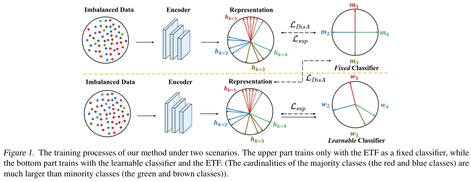
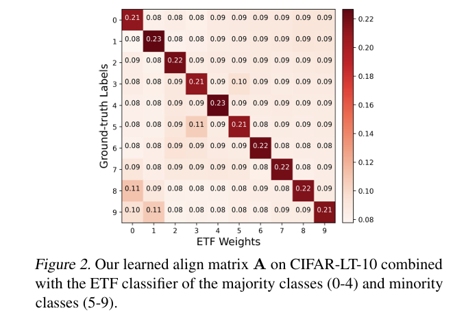
Two Fists, One Heart: Multi-Objective Optimization Based Strategy Fusion for Long-tailed Learning

BibTex
@article{zhao2024moosf,
title={Two Fists, One Heart: Multi-Objective Optimization Based Strategy Fusion for Long-tailed Learning},
author={Zhao, Zhe and Wang, Pengkun and Wen, HaiBin and Xu, Wei and Lai, Song and Zhang, Qingfu and Wang, Yang},
booktitle={Proceedings of the 41st International Conference on Machine Learning},
year={2024}}

url=https://openreview.net/pdf?id=MEZydkOr3l
Summary

The paper presents a novel approach to address the inherent trade-offs in long-tailed learning, where models often perform well on head (frequent) classes at the expense of medium and tail (rare) classes. This imbalance is particularly challenging as existing strategies, such as re-sampling, loss adjustment, and transfer learning, tend to optimize for specific subsets of classes, resulting in a performance trade-off. To resolve this issue, the authors reformulate the problem as a multi-objective optimization (MOO) task, aiming to maximize performance across head, medium, and tail classes simultaneously. They propose a framework called Multi-Objective Optimization based Strategy Fusion (MOOSF) to fuse multiple long-tailed learning strategies effectively, addressing the limitations of single-strategy approaches. MOOSF integrates insights from multi-task learning and multi-objective optimization to balance class-specific performance. The framework begins with a shared feature extraction module that processes input data for all strategies, followed by strategy-specific modules that optimize individual loss functions. Each strategy is weighted dynamically based on its contribution to performance across class groups, using an adaptive weighting mechanism known as Hierarchical Influence Calibrated Adjustment (HICA). HICA evaluates the alignment of each strategy's performance with the overall objective and adjusts weights accordingly, ensuring balanced contributions across all strategies. To resolve conflicts between strategies, MOOSF employs Gradient Harmonization via Orthogonal Projection (GHOP). GHOP adjusts the gradients of conflicting strategies by orthogonalizing them, preventing one strategy from dominating the optimization process. This mechanism ensures that the model explores parameter space efficiently while maintaining harmony between strategies. Additionally, the framework includes Evolving Optimal Strategy Selection (EOSS), which dynamically selects the most effective strategy for each class based on historical performance. By combining these components, MOOSF achieves an efficient and conflict-resolving fusion of strategies, allowing the model to adapt dynamically to the challenges of long-tailed distributions. The authors conducted extensive experiments on benchmark datasets such as CIFAR-100-LT and ImageNet-LT, demonstrating the effectiveness of MOOSF. They found that MOOSF significantly improves overall and class-specific performance compared to individual strategies and traditional multi-task learning. The adaptive fusion approach not only enhances the average performance but also balances the trade-offs between head, medium, and tail classes. Their analysis of gradient harmonization and dynamic weighting shows that these mechanisms effectively reduce conflicts and align strategy contributions, resulting in Pareto-optimal solutions for long-tailed learning.

Problem The paper addresses the problem of balancing performance across head, medium, and tail classes in long-tailed learning by transforming the trade-off challenge into a multi-objective optimization problem and proposing a Multi-Objective Optimization based Strategy Fusion (MOOSF) to integrate and reconcile conflicting strategies for improved generalization.

Images